Adapting 2021 AB 2

Posted on June 29, 2021 by Lin McMullin

Two of nine. Continuing the series started in my last post, this post looks at the AB Calculus 2021 exam question AB 2. The series looks at each question with the aim of showing ways to use the question in with your class as is or by adapting and expanding it. Like most of the AP Exam questions there is a lot more you can ask from the stem and a lot of other calculus you can discuss.

2021 AB 2

This is a Linear Motion Problem (Type 2) and has topics from Unit 4 of the current Course and Exam Description. Two particles are moving on the x-axis and the questions ask about their motion individually and relative to each other. The velocity and initial position are given for each particle. Parts (a), (c), and (d) are typical; (b) is the core of the problem.

The stem is:

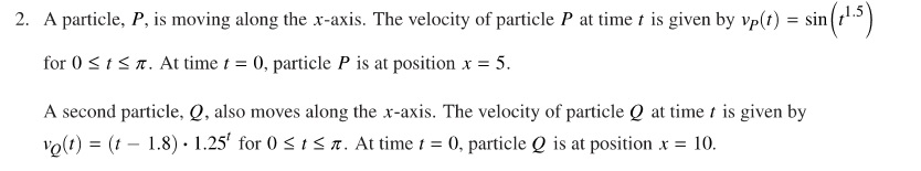
Part (a): Students are asked to find the position of each particle at time t = 1.

Discussion and ideas for adapting this question:

The expected approach is to calculate for each particle the initial position plus the displacement from t = 0 to t = 1. So, for P the computation is $P\left( 1 \right)=5+\int_{0}^{1}{{\sin \left( {{{t}^{{1.5}}}} \right)}}dt$ and similarly for Q(1). This is a calculator allowed question and students should use their calculator to find the answer and not do it by hand.
A different approach is to work it as an initial value differential equation problem. This will work but takes longer than the approach suggested above.
In class, it is worth discussing both methods.
You can adapt this by using a different time.
Another question is to find (only) the displacement if each particle over some time interval. Displacement has been asked in other years.
Ask “Will the particles ever collide? If so when and justify your answer. (Answer: no)

Part (b): Students were asked to determine if the particles are moving apart or towards each other at time t = 1. This is the main question and requires a careful analysis of their motion.

Discussion and ideas for adapting this question:

To determine this, students need to consider the velocity of the particles and their position (from part (a)). P is to the left of Q and moving right. Q is to the right of P and moving left, therefore, the distance between them is decreasing.
You can practice this analysis by using different times.
Ask students to carefully describe the motion of one or both particles: when it is moving left and right, when it changes direction, find the local maximum and minimum positions, etc. Notice that this is really the same as analyzing the shape of a graph. The connection between the two problems will help students understand both better. See: Motion Problems: Same Thing, Different Context

Part (c): A question about speed.

Discussion and ideas for adapting this question:

A typical question. Students should compare the signs of the velocity and acceleration of the particle. If they are the same, the speed is increasing; if different, decreasing.
You may ask this of the other particle.
You may ask this at different times.
See previous posts on speed here and here.

Part (d): Students were required to find the total distanced traveled by Q on the interval [0, π].

Discussion and ideas for adapting this question:

Since speed is the absolute value of the velocity, integrate the absolute value of the velocity. Do this on a calculator.
Adapt this by using a different interval.
Adapt this by using the other particle.
Another (longer) way to approach this question is to find where the particle changes direction by finding where the velocity changes from negative to positive and/or vice versa (i.e., the local extreme values). Then find the distanced traveled on each part of the “trip,” and add or subtract. This will reinforce a lot of the concepts involved in linear motion; that is why it is worth doing. As for the exam, integrating the absolute value is the way to go. However, if this were a non-calculator question, then it would have to be done this way. Find a simpler velocity and try it both ways.
To integrate the absolute value by hand, it is necessary to break the interval into subintervals depending on where the velocity is positive or negative. This is the same as the approach in the bullet immediately above. This, too, is worth showing to reinforce the definition of absolute value.

2021 revised as an in-out question.

There was some unhappiness over the fact that the 2021 AB Calculus exam did not have an in-out questions (Rate and Accumulation Type 1). However, this question does have two rates going in opposite directions. So, just to be ornery, I rewrote it as an in-out questions by changing the context and units while keeping the same velocity functions. The point is that the situation tested can be reframed in other ways. Seeing the same thing in different dress may help students concentrate on the calculus involved. Here it is:

A factory processes cement at the rate of $\displaystyle {{v}_{p}}\left( t \right)=\sin \left( {{{t}^{{1.5}}}} \right)$ tons per hour for $\displaystyle 0\le t\le \pi$ hours. At time t = 0 the amount on hand is P = 5 tons.

The factory ships the cement at a rate given by $\displaystyle {{v}_{Q}}\left( t \right)=\left( {t-1.8} \right){{1.25}^{t}}$ tons per hour for $\displaystyle 0\le t\le \pi$ hours. At time t = 0 the amount shipped is 10 tons.

Find the amount processed and the amount shipped after hour.
Is the amount on hand increasing or decreasing at time t = 1? Explain your reasoning.
At what rate is the rate at which the cement is being shipped changing at t = 1? Is the amount being shipped increasing or decreasing at t = 1? Explain your reasoning.
Find the total amount of cement processed over the time interval $\displaystyle 0\le t\le \pi$ .

Next week 2021 AB 3/ BC 3.

I would be happy to hear your ideas for other ways to use this questions. Please use the reply box below to share your ideas.

Adapting 2021 AB 1 / BC 1

Posted on June 22, 2021 by Lin McMullin

First of nine. One of the things many successful AP Calculus teachers do is to use past AP exam questions throughout the year. Individual multiple-choice exam questions are used as the topics they test are taught; free-response questions are adapted and expanded. There are several ways to do this:

Assign parts of a free-response (FR) question as is as the topic it tests is taught. Later, other parts from the same stem can be assigned. Including previously assigned parts is a spiraling technique. Once students see that you are doing this, they will be more likely to keep up to date on past topics.
Adapting and expanding the questions is another way to use FR questions.

This summer I will be discussing how to do just that. Each week I will look at one of the released 2021 FR questions and suggest how to expand and adapt it. Each stem allows for many more questions than can be asked on any one exam. You have the luxury of asking other things based on the same stem.

This summer’s series of posts will take one question at a time discuss it and suggest additional questions or explorations that may be asked. I will not be presenting solutions. They are available on AP Community bulletin board here and here. I will link the posts to the scoring standards when they are published.

2021 AB 1 / BC 1

This is a Reimann sum and Table question (Type 5) and covers topics from Units 6 and 8 from the current Course and Exam Description. All four parts are fairly typical for this type of problem. There is a little twist in part (b). The context is the density of bacteria growing in a petri dish.

Density is not listed in the Course and Exam Description. It is not covered well in many textbooks. Since it is not listed you need not teach it; exam questions referencing density have enough included information so that a student who has never seen the concept will still be able to answer the question. Keep this in mind as you look at each part; help your students see past the context and look at the calculus. More information on density see these posts Density Functions, and Good Question 15 and Good Question 16.

The stem for 2021 AB 1 / BC 1 reads:

Part (a): Students were asked to estimate the value of the derivative of f at r = 2.25 and explain its meaning, including units, in the context of the problem. The expected procedure is to find the slope between the two values closest to r =2.25. The interpretation is the increase in density as you move away from the center. The units are milligrams per square centimeter per centimeter distant from the center $\frac{{mg/c{{m}^{2}}}}{{cm}}$ .

Discussion and ideas for adapting this question:

AP exams have always asked this question at a value exactly half-way between two values in the table. You may change this to some other place such as r = 3 or r = 0.8.
Units of the derivative are always the units of the function divided by the units of the independent variable. Be sure your students understand this.
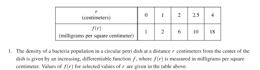
The units can be correctly written as $\frac{{mg}}{{c{{m}^{3}}}}$ , but here is a good change to discuss what the units mean. Why does “milligrams per square centimeter per centimeter distant from the center” make more sense?
Ask “Is there a point in the interval [2, 2.5] where the slope of the tangent line is 8? Justify your answer.” This makes use of the Mean Value Theorem.

Part (b) : As usual in this type of problem, students are asked to write a Riemann sum based on the intervals in the table. The difference here is that the integral being approximated, $\displaystyle 2\pi \int_{0}^{4}{{rf\left( r \right)}}dr$ , has an “extra” factor of r in it.

Discussion and ideas for adapting this question:

The question asked for a right Riemann sum. You can easily adapt this by asking for a left Riemann sum, a midpoint Riemann sum, and/or a Trapezoidal approximation.
You may ask for a Riemann sum without the “extra” factor.
You may find a different Riemann sum problem and include an “extra” factor in it.
The integral is the integral for a radial density function. See the Density blog post cited above, example 2.
The radial density function looks like the integral for finding volumes by the method of cylindrical shells. This is more than a coincidence. Why?

Part (c): This part asked if the answer in (b) is an overestimate or an underestimate, with an explanation. For any approximation, some idea of its accuracy is important. In BC questions on power series approximations, a numerical estimate of the error bound is a common question.

Discussion and ideas for adapting this question:

Ask the same question for a different Riemann sum (left, midpoint, trapezoid).
The error in right and left Riemann sums estimates depend on whether the function is increasing or decreasing, and therefore on the first derivative. Midpoint and Trapezoidal approximation estimates are related to the concavity and therefore to the second derivative. See: Good Question 4)
A visual idea helps keep all this straight. Draw sketches showing the Riemann sum rectangles or trapezoids. Whether they lie above or below the graph of the function determines whether the approximation is an overestimate or underestimate.

Part (d): Typical of the Riemann sum table question is the final part with a related question based on a function and not based on the table.

Discussion and ideas for adapting this question:

This is a calculator allowed question. Students should not try to do the integration by hand.
The question asked for the average value of the function on an interval. Other questions you could ask are find the rate of change (derivative) at a point, the total mass $\int_{1}^{4}{{rf\left( r \right)}}dr$ (note “extra” r), the average rate of change on an interval, etc.

Next week 2021 AB 2.

I would be happy to hear your ideas for other ways to use these questions. Please use the reply box below to share your ideas.

Other Asymptotes

Posted on March 23, 2021 by Lin McMullin

A few days ago, a reader asked if you could find the location of horizontal asymptotes from the derivative of a function. The answer, alas, is no. You can determine that a function has a horizontal asymptote from its derivative, but not where it is. This is because a function and its many possible vertical translations have the same derivative but different horizontal asymptotes. To locate it precisely, we need more information, an initial condition (a point on the curve).

I have written a post about the relationship between vertical asymptotes and the derivative of the function here. Today’s post will discuss horizontal asymptotes and their derivatives.

Definition: a straight line associated with a curve such that as a point moves along an infinite branch of the curve the distance from the point to the line approaches zero and the slope of the curve at the point approaches the slope of the line. (Merriam-Webster dictionary). Thus, asymptotes can be vertical, horizontal, or slanted.

Horizontal Asymptotes

Horizontal asymptotes are a form of end behavior: they appear as $\displaystyle x\to \infty$ or $\displaystyle x\to -\infty$ . Specifically, if a function has a horizontal asymptote(s), then $\displaystyle \underset{{x\to \pm \infty }}{\mathop{{\lim }}}\,{f}'\left( x \right)=0$ , At an asymptote, the curve must approach a horizontal line, therefore its slope must be approaching zero as $\displaystyle x\to \infty$ or $\displaystyle x\to -\infty$ . The converse is not true: If the derivative approaches zero, the function may not have a horizontal asymptote. A counterexample is $\displaystyle f\left( x \right)=\sqrt[3]{x}$ .

In the first four examples that follow, the derivative approaches 0 as $\displaystyle x\to \infty$ and/or $\displaystyle x\to -\infty$ .

Example 1: $\displaystyle {f}'\left( x \right)=\frac{1}{{1+{{x}^{2}}}}$ (Figure 1 in blue).This is the derivative of $\displaystyle f\left( x \right)={{\tan }^{{-1}}}(x),\ -\tfrac{\pi }{2}<f\left( x \right)<\tfrac{\pi }{2}$ . (Figure 1 in red). We see that the derivative approaches zero in both directions, this tells us that there may be horizontal asymptote(s). We must look at the function to find where they are: $\displaystyle y=\tfrac{\pi }{2}$ and $\displaystyle y=-\tfrac{\pi }{2}$

Polar Equations for AP Calculus

Posted on January 26, 2021 by Lin McMullin

A recent thread on the AP Calculus Community bulletin boards concerned polar equations. One teacher observed that her students do not have a very solid understanding of polar graphs when they get to calculus. I expect this is a common problem. While ideally the polar coordinate system should be a major topic in pre-calculus courses, this is sometimes not the case. Some classes may even omit the topic entirely. Getting accustomed to a new coordinate scheme and a different way of graphing is a challenge. I remember not having that good an understanding myself when I entered college (where first-year calculus was a sophomore course). Seeing an animated version much later helped a lot.

This blog post will discuss the basics of polar equations and their graphs. It will not be as much as students should understand, but I hope the basics discussed here will be a help. There are also some suggestions for extending the study of polar function as the end.

Instead of using the Cartesian approach of giving every point in the plane a “name” by giving its distance from the y-axis and the x-axis as an ordered pair (x,y), polar coordinates name the point differently. Polar coordinates use the ordered pair (r, θ), where r, gives the distance of the point from the pole (the origin) as a function of θ, the angle that the ray from the pole (origin) to the point makes with the polar axis, (the positive half of the x-axis).

Start with this Desmos graph. It will help if you open it and follow along with the discussion below. The equation in the example is $\displaystyle r(\theta )=2+4\sin (\theta )$ You may change this to explore other graphs. (Because of the way Desmos graphs, you cannot have a slider for θ; the a-slider will move the line and the point on the graph. r(a) gives the value of r(θ).

Notice that as the angle changes the point at varying distance from the pole traces a curve.
Move the slider to π/6. Since sin(π/6) = 0.5, r(π/6) = 4. The red dot is at the point (4, π/6). Move the slider to other points to see how they work. For example, θ = π/2 gives the point (6,π/2).
When the slider gets to θ = 7π/6, r = 0 and the point is at the pole. After this the values of r are negative, and the point is now on the ray opposite to the ray pointing into the third and fourth quadrants. The dashed line turns red to remind you of this.
As we continue around, the point returns to the origin at θ = 11π/6, then values are again positive.
The graph returns to its starting point when θ = 2π. Note (2,0) is the same point as (2, 2π).
Even though this is the graph of a function, some points may be graphed more than once and the vertical line test does not apply.
If we continued around, the graph will retrace the same path. This often happens when the polar function contains trig functions with integer multiples of θ.
- This does not usually happen if no trig functions are involved – try the spiral r = θ.
- If you enter non-integer multiples of θ and extend the domain to large values, vastly different graphs will appear, often making nice designs. Try $\displaystyle r\left( \theta \right)=2+4\sin \left( {1.3\theta } \right)$ for $\displaystyle 0\le \theta \le 20\pi$ . This is an area for exploration (if you have time).

In pre-calculus courses several families of polar graphs are often studied and named. For example, there are cardioids, rose curves, spirals, limaçons, etc. The AP Exams do not refer to these names and students are not required to know the names. The exception is circles which have the following forms where R is the radius: θ=R, r = Rsin(θ) or r = Rsin(θ)

To change from polar to rectangular for use the equations $x=r\cos \left( \theta \right)$ and $y=r\sin \left( \theta \right)$ . This is simple right triangle trigonometry (draw a perpendicular from the point to the x-axis and from there to the pole).

To change from rectangular to polar form use $r=\sqrt{{{{x}^{2}}+{{y}^{2}}}}$ and $\displaystyle \theta =\arctan \left( {\tfrac{y}{x}} \right)$

AP Calculus Applications

There are two applications that are listed on the AP Calculus Course and Exam Description: using and interpreting the derivative of polar curves (Unit 9.7) and finding the area enclosed by a polar curve(s) (Units 9.8 and 9.9).

Since calculus is concerned with motion, AP Students should be able to analyze polar curves for how things are changing:

The rate of change of r away from or towards the pole is given by $\displaystyle \frac{{dr}}{{d\theta }}$
The rate of change of the point with respect to the x-direction is given by $\displaystyle \frac{{dx}}{{d\theta }}$ where $\displaystyle x=r\cos \left( \theta \right)$ from above.
The rate of change of the point with respect to the y-direction is given by $\displaystyle \frac{{dy}}{{d\theta }}$ where $\displaystyle y=r\sin \left( \theta \right)$ from above.
The slope of the tangent line at a point on the curve is $\displaystyle \frac{{dy}}{{dx}}=\frac{{dy/d\theta }}{{dx/d\theta }}$ . See 2018 BC5 (b)

Area

$\displaystyle \underset{{\Delta \theta \to 0}}{\mathop{{\lim }}}\,\sum\limits_{{i=1}}^{\infty }{{\tfrac{1}{2}}}{{r}_{i}}^{2}\Delta \theta =\tfrac{1}{2}\int_{{{{\theta }_{1}}}}^{{{{\theta }_{2}}}}{{{{r}^{2}}d\theta }}$

CAUTION: In using this formula, we need to be careful that the curve does not overlap itself. In the Desmos example, the smaller loop overlaps the larger loop; integrating from 0 to 2π counts the inner loop twice. Notice how this is handled by considering the limits of integration dividing the region into non-overlapping regions:

The area of the outer loop is $\displaystyle \tfrac{1}{2}\int_{{-\pi /6}}^{{7\pi /6}}{{{{{(2+4\sin (\theta ))}}^{2}}d\theta }}\approx 35.525$
The area of the inner loop is $\displaystyle \tfrac{1}{2}\int_{{7\pi /6}}^{{11\pi /6}}{{{{{(2+4\sin (\theta ))}}^{2}}d\theta }}\approx 2.174$
Integrating over the entire domain gives the sum of these two: $\displaystyle \tfrac{1}{2}\int_{0}^{{2\pi }}{{{{{(2+4\sin (\theta ))}}^{2}}d\theta }}=12\pi \approx 37.699$ . This is not the correct area of either part.

This problem can be avoided by considering the geometry before setting up the integral: make sure the areas do not overlap. Restricting r to only non-negative values is often required by the fine print of the theorem in textbooks, but this restriction is not necessary when finding areas and makes it difficult to find, say, the area of the smaller inner loop of the example. Here is another example:

$\displaystyle r\left( \theta \right)=\cos \left( {3\theta } \right)$ . Between 0 and $\displaystyle 2\pi$ this curve traces the same path twice.

Infinite Sequences and Series – Unit 10

Posted on January 19, 2021 by Lin McMullin

Unit 10 covers sequences and series. These are BC only topics (CED – 2019 p. 177 – 197). These topics account for about 17 – 18% of questions on the BC exam.

Topics 10.1 – 10.2

Topic 10.1: Defining Convergent and Divergent Series.

Topic 10. 2: Working with Geometric Series. Including the formula for the sum of a convergent geometric series.

Topics 10.3 – 10.9 Convergence Tests

The tests listed below are tested on the BC Calculus exam. Other methods are not tested. However, teachers may include additional methods.

Topic 10.3: The n^th Term Test for Divergence.

Topic 10.4: Integral Test for Convergence. See Good Question 14

Topic 10.5: Harmonic Series and p-Series. Harmonic series and alternating harmonic series, p-series.

Topic 10.6: Comparison Tests for Convergence. Comparison test and the Limit Comparison Test

Topic 10.7: Alternating Series Test for Convergence.

Topic 10.8: Ratio Test for Convergence.

Topic 10.9: Determining Absolute and Conditional Convergence. Absolute convergence implies conditional convergence.

Topics 10.10 – 10.12 Taylor Series and Error Bounds

Topic 10.10: Alternating Series Error Bound.

Topic 10.11: Finding Taylor Polynomial Approximations of a Function.

Topic 10.12: Lagrange Error Bound.

Topics 10.13 – 10.15 Power Series

Topic 10.13: Radius and Interval of Convergence of a Power Series. The Ratio Test is used almost exclusively to find the radius of convergence. Term-by-term differentiation and integration of a power series gives a series with the same center and radius of convergence. The interval may be different at the endpoints.

Topic 10.14: Finding the Taylor and Maclaurin Series of a Function. Students should memorize the Maclaurin series for $\displaystyle \frac{1}{{1-x}}$ , sin(x), cos(x), and e^x.

Topic 10.15: Representing Functions as Power Series. Finding the power series of a function by, differentiation, integration, algebraic processes, substitution, or properties of geometric series.

Timing

The suggested time for Unit 9 is about 17 – 18 BC classes of 40 – 50-minutes, this includes time for testing etc.

Previous posts on these topics:

Before sequences

Amortization Using finite series to find your mortgage payment. (Suitable for pre-calculus as well as calculus)

A Lesson on Sequences An investigation, which could be used as early as Algebra 1, showing how irrational numbers are the limit of a sequence of approximations. Also, an introduction to the Completeness Axiom.

Everyday Series

Convergence Tests

Reference Chart

Which Convergence Test Should I Use? Part 1 Pretty much anyone you want!

Which Convergence Test Should I Use? Part 2 Specific hints and a discussion of the usefulness of absolute convergence

Good Question 14 on the Integral Test

Sequences and Series

Graphing Taylor Polynomials Graphing calculator hints

Introducing Power Series 1

Introducing Power Series 2

Introducing Power Series 3

New Series from Old 1 substitution (Be sure to look at example 3)

New Series from Old 2 Differentiation

New Series from Old 3 Series for rational functions using long division and geometric series

Geometric Series – Far Out An instructive “mistake.”

A Curiosity An unusual Maclaurin Series

Synthetic Summer Fun Synthetic division and calculus including finding the (finite)Taylor series of a polynomial.

Error Bounds

Error Bounds Error bounds in general and the alternating Series error bound, and the Lagrange error bound

The Lagrange Highway The Lagrange error bound.

What’s the “Best” Error Bound?

Review Notes

Type 10: Sequences and Series Questions

Contextual Applications of the Derivative – Unit 4

Posted on September 22, 2020 by Lin McMullin

Unit 4 covers rates of change in motion problems and other contexts, related rate problems, linear approximation, and L’Hospital’s Rule. (CED – 2019 p. 82 – 90). These topics account for about 10 – 15% of questions on the AB exam and 6 – 9% of the BC questions.

You may want to consider teaching Unit 5 (Analytical Applications of Differentiation) before Unit 4. Notes on Unit 5 will be posted next Tuesday September 29, 2020

Topics 4.1 – 4.6

Topic 4.1 Interpreting the Meaning of the Derivative in Context Students learn the meaning of the derivative in situations involving rates of change.

Topic 4.2 Linear Motion The connections between position, velocity, speed, and acceleration. This topic may work better after the graphing problems in Unit 5, since many of the ideas are the same. See Motion Problems: Same Thing, Different Context

Topic 4.3 Rates of Change in Contexts Other Than Motion Other applications

Topic 4.4 Introduction to Related Rates Using the Chain Rule

Topic 4.5 Solving Related Rate Problems

Topic 4.6 Approximating Values of a Function Using Local Linearity and Linearization The tangent line approximation

Topic 4.7 Using L’Hospital’s Rule for Determining Limits of Indeterminate Forms. Indeterminate Forms of the type $\displaystyle \tfrac{0}{0}$ and $\displaystyle \tfrac{\infty }{\infty }$ . (Other forms may be included, but only these two are tested on the AP exams.)

Topic 4.1 and 4.3 are included in the other topics, topic 4.2 may take a few days, Topics 4.4 – 4.5 are challenging for many students and may take 4 – 5 classes, 4.6 and 4.7 two classes each. The suggested time is 10 -11 classes for AB and 6 -7 for BC. of 40 – 50-minute class periods, this includes time for testing etc.

This is a re-post and update of the third in a series of posts from last year. It contains links to posts on this blog about the differentiation of composite, implicit, and inverse functions for your reference in planning. Other updated post on the 2019 CED will come throughout the year, hopefully, a few weeks before you get to the topic.

Posts on these topics include:

Motion Problems

Motion Problems: Same Thing, Different Context

Speed

A Note on Speed

Related Rates

Graph Analysis Questions (Type 3)

Posted on March 10, 2020 by Lin McMullin

AP Questions Type 3: Graph Analysis

The long name is “Here’s the graph of the derivative, tell me things about the function.”

Students are given either the equation of the derivative of a function or a graph identified as the derivative of a function with no equation is given. It is not expected that students will write the equation of the function from the graph (although this may be possible); rather, students are expected to determine important features of the function directly from the graph of the derivative. They may be asked for the location of extreme values, intervals where the function is increasing or decreasing, concavity, etc. They may be asked for function values at points. They will be asked to justify their conclusions.

The graph may be given in context and student will be asked about that context. The graph may be identified as the velocity of a moving object and questions will be asked about the motion. See Linear Motion Problems (Type 2)

Less often the function’s graph may be given and students will be asked about its derivatives.

What students should be able to do:

Read information about the function from the graph of the derivative. This may be approached by derivative techniques or by antiderivative techniques.
Find and justify where the function is increasing or decreasing.
Find and justify extreme values (1^st and 2^nd derivative tests, Closed interval test a/k/a Candidates’ test).
Find and justify points of inflection.
Find slopes (second derivatives, acceleration) from the graph.
Write an equation of a tangent line.
Evaluate Riemann sums from geometry of the graph only. This usually involves familiar shapes such as triangles or semicircles.
FTC: Evaluate integral from the area of regions on the graph.
FTC: The function, g(x), maybe defined by an integral where the given graph is the graph of the integrand, f(t), so students should know that if,

$\displaystyle g\left( x \right)=g\left( a \right)+\int_{a}^{t}{f\left( t \right)dt}$ then ${g}'\left( x \right)=f\left( x \right)$ and ${{g}'}'\left( x \right)={f}'\left( x \right)$ .

In this case, students should write ${g}'(t)=f\left( t \right)$ on their answer paper, so it is clear to the reader that they understand this.

Not only must students be able to identify these things, but they are usually asked to justify their answer and reasoning. See Writing on the AP Exams for more on justifying and explaining answers.

The ideas and concepts that can be tested with this type question are numerous. The type appears on the multiple-choice exams as well as the free-response. Between multiple-choice and free-response this topic may account for 15% or more of the points available on recent tests. It is very important that students are familiar with all the ins and outs of this situation.

As with other questions, the topics tested come from the entire year’s work, not just a single unit. In my opinion many textbooks do not do a good job with integrating these topics, so be sure to use as many actual AP Exam questions as possible. Study past exams; look them over and see the different things that can be asked. The Graph Analysis problem may cover topics primarily from primarily from Unit 4, Unit 5, and Unit 8 of the 2019 CED

For some previous posts on this subject see October 15, 17, 19, 24, 26 (my most read post), 2012 and January 25, 28, 2013

Free-response questions:

Function given as a graph, questions about its integral (so by FTC the graph is the derivative): 2016 AB 3/BC 3, 2018 AB3
Table and graph of function given, questions about related functions: 2017 AB 6,
Derivative given as a graph: 2016 AB 3 and 2017 AB 3
Information given in a table 2014 AB 5

Multiple-choice questions from non-secure exam. Notice the number of questions all from the same year; this is in addition to one free-response question (~25 points on AB and ~23 points on BC out of 108 points total)

2012 AB: 2, 5, 15, 17, 21, 22, 24, 26, 76, 78, 80, 83, 82, 84, 85, 87
2012 BC 3, 11, 12, 15, 12, 18, 21, 76, 78, 80, 81, 84, 88, 89

A good activity on this topic is here. The first pages are the teacher’s copy and solution. Then there are copies for Groups A, B, and C. Divide your class into 3 or 6 or 9 groups and give one copy to each. After they complete their activity have the students compare their results with the other groups.

Revised March 12, 2021

Teaching Calculus

The pleasure lies not in discovering the truth, but in searching for it.

Category Archives: Derivative Applications

Adapting 2021 AB 2

2021 AB 2

Adapting 2021 AB 1 / BC 1

2021 AB 1 / BC 1

Other Asymptotes

Polar Equations for AP Calculus