My Favorite Function

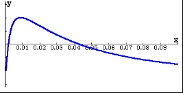
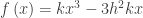
My favorite function is f\left( x \right)=\sin \left( \ln \left( x \right) \right). I like to ask folks how many zeros this function has on the interval 0<x\le 1.

Most folks will get their calculator out and graph the function on the interval

Fav 1

Two zeros: one at 1 and the other about 0.05 more or less.

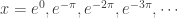
So then I suggest they look at 0<x\le 0.1. This is the left 10% of the first window.

Fav 2

Sure enough there is the zero near 0.05 but there is another near 0

So another window 0<x\le 0.01

Fav 3

Pretty soon they get the idea. Every time we stretch out the graph, there are more roots.

What is going on? The first thing is that this is not a question to be answered on a graphing calculator, the nice graphs notwithstanding.

So try to solve it by hand. Since \sin \left( x \right)=0 for x=k\pi  where k is an integer, we need to see when \ln \left( x \right)=k\pi . That will be when \displaystyle x={{e}^{k\pi }}. And since our domain is proper fractions it must be that k\le 0. So the zeros are infinite in number, namely \displaystyle x={{e}^{0}},{{e}^{-\pi }},{{e}^{-2\pi }},{{e}^{-3\pi }},\cdots . Which answers the original question but raises others.

Why can’t we see the zeros on the graph?

This is not a calculator glitch; in fact computers can do no better. Each root is the next largest root divided by \displaystyle {{e}^{\pi }}\approx 23. So each root is about \displaystyle \tfrac{1}{23}of the larger next root.

The calculator screen is made up of pixels. The number you choose for xmin is the center of the column of pixels; the number you choose for xmax is the center of the right-most column of pixels. The distance between the two ends is divided and assigned evenly to the centers of the other columns of pixels. The y-coordinates of the pixels are calculated the same way. The calculator evaluates the function at each pixel value and turns on the pixel in that column closest to (rarely at) the function’s value. A lot can go on between the pixels and the graphing calculator and its operator will not see what is happening there.

In this example, all the missing roots are between the first and second pixels on the left! When you change xmax to see the left 10% of the screen you see one and every now and then two roots, but the rest are still between the two pixels on the left.

Would a wider screen help? Perhaps a little, but not much.

Here’s a good exercise for a class: Suppose you could print the graph on a paper 1 mile (5280 feet) wide with the root at x = 1 on the right edge. Where would the next several roots be?

  •  \displaystyle {{e}^{-\pi }} is 228.169 feet from the left edge
  •  \displaystyle {{e}^{-2\pi }} is 9.860 feet from the left edge
  •  \displaystyle {{e}^{-3\pi }} is 0.426 feet or 5.113 inches from the left edge
  •  \displaystyle {{e}^{-4\pi }} is 0.221 inches from the left edge (less than ¼ inch)
  • And all the remaining roots are within 0.00955 inches from the left edge.

If the paper stretched from the earth to the sun you could see a few more. At 93,000,000 miles, the zero at \displaystyle {{e}^{-10\pi }} is about 0.134 inches from the edge.

So why do I like this problem?

Look at all the math we did.

  • We learned that graphing is not always the path to the answer.
  • We learned how calculators choose the points they graph, and which they miss.
  • We practiced how to solve a trig equation.
  • We practiced how to solve a natural logarithm equation.
  • We consider the actual size of the negative powers of e and saw how they got exponentially smaller.
  • We did a practical problem in scaling to illustrate how fast the numbers diminish.

Why do I like this function?

What’s not to like?

Update (February 7, 2015) Chip Rollinson made this cool Geogebra applet to illustrate My Favorite Function. Use the slider on the screen and notice the x-axis scale as it changes. Thank you, Chip. 


August

This note will stay on top for a while

New posts will appear below. 

Today this blog is one year old. Thanks to all of you who have been following it. I hope you have found things here that help you and your students. During the first year I gave suggestions on teaching the content of a first-year calculus course. This does not change much from year to year so the post are still here and can be found using the “Posts by Topic” and “Archive” links on the right side of the screen and the “Tags” cloud at the bottom of the screen. There is also a new page called “Thru the Year” at the top. Here you will find a list of the topics in order by month. I will add a month each month.

This coming year I will try to fill in with the topics I have not already posted about. Suggestions are always welcome.

I continue my un-retirement this year by returning to teaching high school AP calculus BC along with Algebra 1. That may make for some interesting posts.

Hope you enjoy the new pictures.

I hope you have a  good year; wish me luck on mine.

Modified Tabular Integration

Several weeks ago, Dr. Qibo Jing, an AP teacher at Rancho Solano Preparatory School in Scottsdale, Arizona, posted a new way to approach tabular integration to the AP Calculus Community discussion group.  He calls this the Modified Tabular Method. The algorithm makes repeated integration by parts quicker and more streamlined than the usual method. The usual method is explained here.

Here is Dr. Jing’s method outlined and illustrated with this example \displaystyle I=\int{\left( {{x}^{3}}+7{{x}^{2}} \right)\cos \left( x \right)dx}

Step 1: Identify u and dv in the usual way and rewrite the given integral in terms of u={{x}^{3}}+7{{x}^{2}} and dv=\cos \left( x \right)=\tfrac{d}{dx}\sin \left( x \right).

\displaystyle I=\int{\left( {{x}^{3}}+7{{x}^{2}} \right)\cos \left( x \right)dx}=\int{\left( {{x}^{3}}+7{{x}^{2}} \right)\left( \tfrac{d}{dx}\left( \sin x \right) \right)}

Step 2: The first term of the antiderivative is the product of the two functions that appear in the revised integral:

\displaystyle I=\int{\left( {{x}^{3}}+7{{x}^{2}} \right)\left( \tfrac{d}{dx}\left( \sin x \right) \right)}=\left( {{x}^{3}}+7{{x}^{2}} \right)\sin \left( x \right)\cdots

Step 3: The remaining terms alternate sign. The next term has subtraction sign etc. The first factor of the next term is the derivative of the first factor of the current term. The second factor is the antiderivative of the second factor of the current term – differentiate the first factor; integrate the second factor.

\displaystyle I =\int{\left( {{x}^{3}}+7{{x}^{2}} \right)\left( \tfrac{d}{dx}\left( \sin x \right) \right)}=\left( {{x}^{3}}+7{{x}^{2}} \right)\sin \left( x \right)-\left( 3{{x}^{2}}+14x \right)\left( -\cos \left( x \right) \right)\cdots

Step 4: Alternate signs and repeat step 3 until the term becomes zero or until the original form appears (See next example). DO NOT simplify either factor until you are done as this may change later terms.

Modified A

The simplified result is

\displaystyle I=\left( {{x}^{3}}+7{{x}^{2}}-6x-14 \right)\sin \left( x \right)+\left( 3{{x}^{2}}+14x-6 \right)\cos \left( x \right)+C

Here is a second example.  In this example the original integral returns as the third term.

\displaystyle I=\int{{{e}^{x}}\sin \left( x \right)dx=\int{\sin \left( x \right)\left( \tfrac{d}{dx}{{e}^{x}}dx \right)}}

=\sin \left( x \right)\left( {{e}^{x}} \right)-\cos \left( x \right)\left( {{e}^{x}} \right)+\left( -\sin \left( x \right) \right)\left( {{e}^{x}} \right)

={{e}^{x}}\sin \left( x \right)-\cos \left( x \right)\left( {{e}^{x}} \right)-I

2I={{e}^{x}}\sin \left( x \right)-\cos \left( x \right)\left( {{e}^{x}} \right)

I=\tfrac{1}{2}\left( {{e}^{x}}\sin \left( x \right)-\cos \left( x \right)\left( {{e}^{x}} \right) \right)+C

This really is a simpler algorithm than the usual tabular method.

More Gold

Last week I discussed Lin McMullin’s Theorem (that would be me). The theorem finds where the Golden Ratio shows up in any fourth-degree polynomial.  Shortly after that began making the rounds, I got an e-mail from David Tschappat who was then a senior in college. He is now a doctoral student working for an online learning solutions provider. 

He related the discovery of a similar appearance of the Golden Ratio in cubic polynomials! Here is his theorem and two other related facts about cubic polynomials (lemmas really) as developed by me.

All cubic polynomials are symmetric to their point of inflection. Therefore, we can simplify matters by translating any cubic so that its point of inflection is at the origin. The general equation will then be f\left( x \right)=k{{x}^{3}}-3{{h}^{2}}kx.

I choose this rather unusual form so that the x-coordinates of the extreme points will be “nice” variables, namely h and –h the zeros of {f}'\left( x \right)=3k{{x}^{2}}-3{{h}^{2}}k=3k\left( x-h)(x+h \right). The leading coefficient k will eventually divide out and not be a concern.

Now consider two other values x = –2h and x = 2h. So, assuming h > 0, there are five evenly spaced values -2h<-h<0<h<2h that we will consider.

The first two results I will leave as an exercise, as they say:

  1. f\left( -2h \right)=f\left( h \right) and f\left( -h \right)=f\left( 2h \right)
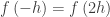
. This means that the extreme values are the same as a point on the graph 3h units away on the other side of the y-axis. This is mildly interesting in itself. The reason it is mentioned id that we will use these points soon.
  2. {f}'\left( -2h \right)={f}'\left( 2h \right) which is really true for any points at equal distances on opposite sides of the origin. This is obvious from the symmetry of the cubic.

Now comes the interesting and strange part. An equation of a line through one extreme point with a slope equal to that at the point with the same y-coordinate on the other side of the origin (or for that matter the point h units farther away on the same side of the y-axis) is

y=f\left( -h \right)+{f}'\left( 2h \right)\left( x-\left( -h \right) \right)

y=\left( k{{\left( -h \right)}^{3}}-3{{h}^{2}}k\left( -h \right) \right)+\left( 3k{{\left( 2h \right)}^{2}}-3{{h}^{2}}k \right)\left( x+h \right)

y=k\left( 11{{h}^{3}}+9{{h}^{2}}x \right)

Now find where this line intersect the original cubic by solving y=f\left( x \right). The equation can be solved by hand. We know that x = h is one solution. Synthetic division will give a quadratic and the quadratic formula will do the rest.

k\left( 11{{h}^{3}}+9{{h}^{2}}x \right)=k{{x}^{3}}-3{{h}^{2}}kx

0={{x}^{3}}-12{{h}^{2}}x-11{{h}^{3}}

0=\left( x-h \right)\left( {{x}^{2}}+hx-11{{h}^{2}} \right)

\displaystyle x=h,\frac{1+3\sqrt{5}}{2}h,\frac{1-3\sqrt{5}}{2}h

What? You were expecting the Golden Ratio? Not to worry; it’s there!

\displaystyle \Phi \left( -h \right)+\phi \left( 2h \right)=\frac{1+\sqrt{5}}{2}\left( -h \right)+\frac{1-\sqrt{5}}{2}\left( 2h \right)=\frac{1-3\sqrt{5}}{2}h

\displaystyle \Phi \left( 2h \right)+\phi \left( -h \right)=\frac{1+\sqrt{5}}{2}\left( 2h \right)+\frac{1-\sqrt{5}}{2}\left( -h \right)=\frac{1+3\sqrt{5}}{2}h

Where \displaystyle \Phi =\frac{1+\sqrt{5}}{2} 
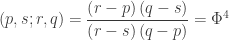
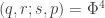
is the Golden Ratio and \displaystyle \phi ={{\Phi }^{-1}}=\frac{1-\sqrt{5}}{2} 
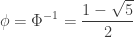
is the reciprocal of the Golden Ratio.

A similar computation using the other extreme point gives similar results.

Yes, the Golden Ratio is there; I don’t know why it should be there, but it is.

Thank you, David.

Lin McMullin’s Theorem

Mathematics more often tends to delight when it exhibits an unanticipated result rather than conforming to … expectations. In addition, the pleasure derived from mathematics is related in many cases to the surprise felt upon the perception of totally unexpected relationships and unities.

– Mario Livio, The Golden Ratio

I have a theorem named after me. I did not name it, but I did prove it – well more like I tripped over it. It is a calculus related idea. Here is how it came about. I say “came about” because as you will see I did not set out to prove it. I just sort of fell in my lap as I was working on something else.

I was trying to do an animation of an idea that I had heard about: If you have a fourth degree, or quartic, polynomial with a “W” shape it has two points of inflection. If you draw a line through the points of inflection three regions enclosed by the line and the polynomial’s graph are formed. The areas of these regions are in the ratio of 1:2:1. In order to make the animation work I needed the general coordinates of the four points where the line intersects the quartic.

The straightforward way to proceed would be to write a general fourth degree polynomial,

f\left( x \right)={{c}_{4}}{{x}^{4}}+{{c}_{3}}{{x}^{3}}+{{c}_{2}}{{x}^{2}}+{{c}_{1}}x+{{c}_{0}}

differentiate it twice to find the second derivative. Then find the zeros of the second derivative (by the quadratic formula), write the equation of the line through them, and then find where else the line intersects the quartic. Without even starting I realized that even with a CAS the algebra and equation solving was going to be really fun (Not!). So, I decided on an alternative approach.

I decided to let the zeros of the second derivative be x = a and x = b, then at least they would be easy to work with. Then the second derivative is \displaystyle {{f}'}'\left( x \right)=12{{c}_{4}}\left( x-a \right)\left( x-b \right) where the {{c}_{4}}  is the leading coefficient of the quartic and the 12 comes from differentiating twice.

I integrated to get the first derivative and added {{c}_{1}}, the coefficient of the linear term, as the constant of integration. I integrated again and added {{c}_{0}}, the constant term. as the constant of integration. This resulted in the original quartic function:

\displaystyle f\left( x \right)={{c}_{4}}{{x}^{4}}-2\left( a+b \right){{c}_{4}}{{x}^{3}}+6ab{{c}_{4}}{{x}^{2}}+{{c}_{1}}x+{{c}_{0}}

Then I wrote the equation of y(xthe line through the points of inflection. It is too long to copy, but you may see it in the screen capture at the end of the post. (That is what is nice about a CAS: you really do not have to worry about how complicated things are.)

Then I solved the equation f\left( x \right)=y\left( x \right)
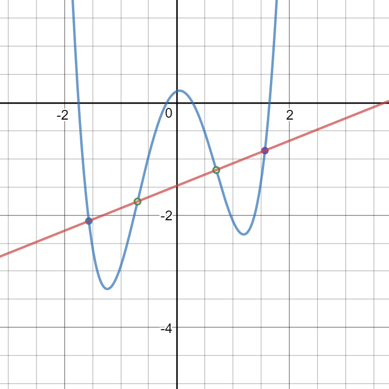
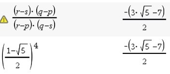
. Two of the solutions are x = a and x = b as I expected. (This means that you could do synthetic division by hand since you know two of the roots.) The other two I did not expect. They are:

\displaystyle {{x}_{1}}=\frac{1+\sqrt{5}}{2}a+\frac{1-\sqrt{5}}{2}b and \displaystyle {{x}_{2}}=\frac{1+\sqrt{5}}{2}b+\frac{1-\sqrt{5}}{2}a

And that’s when I stopped astonished! Those numbers are the Golden Ratio \Phi =\frac{1+\sqrt{5}}{2}
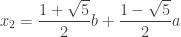
,  and its reciprocal \phi ={{\Phi }^{-1}}=\frac{1-\sqrt{5}}{2}. So the roots are \Phi a+\phi b and \Phi b+\phi a. How did they get there?

To this day I have no idea why the Golden Ratio should be so involved with quartic polynomials, but there they are in every quartic!

There were no assumptions made about a and b – they could be Complex numbers. In that case there are no points of inflection, but the “line” and the quartic still will have the same value at the four points.

October 16, 2022 Update: If the solutions of \displaystyle {y}''=0 are the Complex conjugates \displaystyle a=\alpha +\beta i and \displaystyle b=\alpha -\beta i then \displaystyle {{x}_{1}}=\alpha +\sqrt{5}\beta i and \displaystyle {{x}_{2}}=\alpha -\sqrt{5}\beta i. When graphed on an Argand diagram the four points are collinear on the vertical line at \displaystyle x=\alpha

This was all in 2013 and until just this year I never checked the ratio of the areas. (They check.)

Here is a CAS printout of the entire computation.LMT 2

An interactive Desmos demo of this can be found here


October 16, 2022, Update: If the solutions of \displaystyle {y}''=0 are the Complex conjugates \displaystyle a=\alpha +\beta i and \displaystyle b=\alpha -\beta i then \displaystyle {{x}_{1}}=\alpha +\sqrt{5}\beta i and \displaystyle {{x}_{2}}=\alpha -\sqrt{5}\beta i. When graphed on an Argand diagram the four points are collinear on the vertical line at \displaystyle x=\alpha


November 10, 2020, Update: I received an email this week form Dominique Laurain, a computer science and applied math engineer from France, who describes himself as a mathematics hobbyist. He discovered another interesting relationship between the coordinates of the x-coordinates of the four points on the line described above. The four points on the line through the points of inflection of a fourth degree polynomial with Real roots in the drawing above from left to right are p, q, r, and s. The coordinates of the points of inflection are a and as in the post above.  

One, of several, cross-ratios of four points with x-coordinates of p, q r, and s is defined as

\displaystyle (p,s;r,q)=\frac{{\left( {r-p} \right)\left( {q-s} \right)}}{{\left( {r-s} \right)\left( {q-p} \right)}}.

Dominique Laurin discovered that \displaystyle (p,s;r,q)=\frac{{\left( {r-p} \right)\left( {q-s} \right)}}{{\left( {r-s} \right)\left( {q-p} \right)}}={{\Phi }^{4}}

The computation is shown in the figure below.

There are 24 other cross-ratios depending on the order of the points. In groups of 4, the 24 possible orders are equal to 6 related values. See the cross-ratio link above above. For example, the cross-ratio in the order (s, p; r, q) is {{\varphi }^{4}}

Also, (q,r;s,p)={{\Phi }^{4}}


Other interesting information:

The Golden Ratio also appears in cubic equations. See the Tashappat – McMullin theorem here.

Quartic Polynomials and the Golden Ratio” by Harald Totland of the Royal Norwegian Naval Academy. (June 2009)

Speaking of the Golden Ratio, the Calculus Humor website has a nice feature on the Golden Ratio in logos. To view it click here.

Link for cross-ratios

Revised and updated July 20 and 23, 2017, November 10, 2020


Experimenting with CAS – Chain Rule

Discovering things in mathematics can be facilitated by using a computer algebra system (CAS) available on many handheld calculators and computer apps. A CAS can provide good data with which to draw conclusions. You can do “experiments” by producing the results with a CAS and looking for patterns. As an example, let’s look at how you and your students might discover the chain rule for derivatives.

One of the ways you could introduce the chain rule is to ask your class to differentiate something like (3x + 7)2. Not knowing about the chain rule, just about the only way to proceed is to expand the expression to 9x2 + 42x + 49 and differentiate that: 18x + 42 and then factor 6(3x + 7). Then you show how this relates to the power rule and where the “extra” factor of 3 comes from differentiating the (3x + 7).  You really cannot a much more complicated example, say a third or fourth power, because the algebra gets complicated very fast.

Or does it?

Suggest your students use a CAS to do the example above this time using the third power. The output might look like this:

CAS A

But even better: what we want is just the answer. Who cares about all the algebra in between? Try a few powers until the pattern become obvious.

CAS B

Now we have some good data to work with. Can you guess the pattern?

Nor sure where the “extra” factor of 3 comes from? Try changing the 3 in the original and keep the exponent the same.

CAS C

Now can you guess the chain rule? See if what you thought is right by changing only the inside exponent.

CAS G

Then you can try some others:

CAS D

You can count on the CAS giving you the correct data (answers). Do enough experiments until the chain rule pattern becomes clear.

But I think the big thing is not the chain rule, but that the students are learning how to experiment in mathematics situations. In these we started by changing only the outside power. Then we kept the power the same power and changed the coefficient of the linear factor. Then we changed the power inside power, each time seeing if our tentative rule for differentiating composite function was correct and adjusting it if it was not. Finally we tried a variety of different expressions. You change things. Not big things but little things. You don’t jump from one trial to something very different, only something a little different.

You can do the same thing for the product rule, the quotient rule, maybe some integration rules and so on. You have accomplished your goal when the students can produce the data they need without your suggestions.

But be aware: sometimes this can lead to unexpected results. Does the pattern hold here?

CAS E

Or here?

CAS F

Hint: \frac{7}{3.2}=2.1875  and 3{{\left( 3.2 \right)}^{3}}=98.304


Revised 8-25-17

Variations on a Theme – 2

This is the second in an occasional series on adapting and expanding AP calculus exam questions. Variations on multiple-choice questions may make other multiple-choice questions, or, if you do not like making up all the “wrong” choices they can be changed to short answer questions for use in your class homework or test. Other variations make for good discussion questions.

 Today we will take a look at 2008 AB 10. This question gave the graph below and asked which of \displaystyle \int_{1}^{3}{f\left( x \right)dx}, a left, right, or midpoint Riemann sum approximation, or a trapezoidal sum approximation of the integral all with four subintervals of equal length has the least value.

Variations 2 pix 1

I’ll refer to these as I, L, R, M and T. The answer is R as a quick sketch will show.

In the discussion we will assume the curve does not change direction or concavity over the interval of integration. The answers to the questions in the variations are at the end of this post.

Variation 1: The question seems pretty easy so let’s beef it up a bit. How about asking the student to put I, L, R, M and T in order from smallest to largest? For a multiple-choice question answer choices are inequalities with all 5 sums in them.

The midpoint Riemann sum may be the most difficult to see. Here is the way to explain it. See the figure below.

Variations 2 pix 2

On each subinterval draw the horizontal segment at the function value at the midpoint of the interval. At this same point draw a tangent segment from one side of the interval to the other. This forms two congruent triangles with the horizontal segment and the edges of the interval.

Therefore, this midpoint trapezoid and the midpoint rectangle have the same area. Then because of the concavity, we see that in this case the midpoint Riemann sum, M, will be larger than the integral, I. With the same concavity the trapezoidal approximation will lie below the curve and therefore T < I < M. This will be true for any curve that is concave down. The opposite is true for a curve that is concave up: M < I < T. M and T are always on opposite sides of I. 

Variation 2: Change the number of subintervals, but keep the same number for each sum. Does this change anything?

Variation 3: Change the number of subintervals so that the sums over the same interval have a different number of subintervals. Does this change anything?

Variation 4: Change the shape of the curve to one of the other 4 shapes that a curve may have. How does this change the order of the sums?

Variation 5: Move the graph from above the ­x-axis to below. Does this change anything?

Variation 6: The reversal problem. Suppose that L < T < I < M < R; describe the shape of the curve. Other orders can be used as well. In fact this idea has appeared on an AP calculus exams. In 2003 AB 85 students were told that a trapezoidal sum over approximates and a right Riemann sum under approximates a certain integral. The question asked which of 5 graphs could be the graph of the function.

___________________

If you have other variations please click “Leave a Comment” to share them. If you have variations on a different question please share them as well.

___________________

Answers:

Variation 1: R < T < I < M < L

Variation 2: No. Since the order will be the same on each subinterval adding them will not change the order.

Variation 3: This makes a difference. In the first figure above, consider a trapezoidal sum with one subinterval compared to a right Riemann sum with many subintervals. The right Riemann sum will be very close to the integral with its rectangles ending above the trapezoidal segment between the endpoints. In this case T < R for the figure shown.

Variation 4: The left and right Riemann sums depend on whether the curve is decreasing or increasing. The Trapezoidal sum and the midpoint Riemann sum depend on the concavity. For example, an increasing concave up curve the order is L < M < I < T < R.

Variation 5: No. If the curve is entirely below the x-axis all the values will be negative, but all the results discussed in the other variations will be the same; the order will not change.

Variation 6: The curve is increasing and concave down.