exponential function | Teaching Calculus

My favorite function is $f\left( x \right)=\sin \left( \ln \left( x \right) \right)$ . I like to ask folks how many zeros this function has on the interval $0<x\le 1$ .

Most folks will get their calculator out and graph the function on the interval

Two zeros: one at 1 and the other about 0.05 more or less.

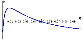
So then I suggest they look at $0<x\le 0.1$ . This is the left 10% of the first window.

Sure enough there is the zero near 0.05 but there is another near 0

So another window $0<x\le 0.01$

Pretty soon they get the idea. Every time we stretch out the graph, there are more roots.

What is going on? The first thing is that this is not a question to be answered on a graphing calculator, the nice graphs notwithstanding.

So try to solve it by hand. Since $\sin \left( x \right)=0$ for $x=k\pi$ where k is an integer, we need to see when $\ln \left( x \right)=k\pi$ . That will be when $\displaystyle x={{e}^{k\pi }}$ . And since our domain is proper fractions it must be that $k\le 0$ . So the zeros are infinite in number, namely $\displaystyle x={{e}^{0}},{{e}^{-\pi }},{{e}^{-2\pi }},{{e}^{-3\pi }},\cdots$ . Which answers the original question but raises others.

Why can’t we see the zeros on the graph?

This is not a calculator glitch; in fact computers can do no better. Each root is the next largest root divided by $\displaystyle {{e}^{\pi }}\approx 23$ . So each root is about $\displaystyle \tfrac{1}{23}$ of the larger next root.

The calculator screen is made up of pixels. The number you choose for xmin is the center of the column of pixels; the number you choose for xmax is the center of the right-most column of pixels. The distance between the two ends is divided and assigned evenly to the centers of the other columns of pixels. The y-coordinates of the pixels are calculated the same way. The calculator evaluates the function at each pixel value and turns on the pixel in that column closest to (rarely at) the function’s value. A lot can go on between the pixels and the graphing calculator and its operator will not see what is happening there.

In this example, all the missing roots are between the first and second pixels on the left! When you change xmax to see the left 10% of the screen you see one and every now and then two roots, but the rest are still between the two pixels on the left.

Would a wider screen help? Perhaps a little, but not much.

Here’s a good exercise for a class: Suppose you could print the graph on a paper 1 mile (5280 feet) wide with the root at x = 1 on the right edge. Where would the next several roots be?

$\displaystyle {{e}^{-\pi }}$ is 228.169 feet from the left edge
$\displaystyle {{e}^{-2\pi }}$ is 9.860 feet from the left edge
$\displaystyle {{e}^{-3\pi }}$ is 0.426 feet or 5.113 inches from the left edge
$\displaystyle {{e}^{-4\pi }}$ is 0.221 inches from the left edge (less than ¼ inch)
And all the remaining roots are within 0.00955 inches from the left edge.

If the paper stretched from the earth to the sun you could see a few more. At 93,000,000 miles, the zero at $\displaystyle {{e}^{-10\pi }}$ is about 0.134 inches from the edge.

So why do I like this problem?

Look at all the math we did.

We learned that graphing is not always the path to the answer.
We learned how calculators choose the points they graph, and which they miss.
We practiced how to solve a trig equation.
We practiced how to solve a natural logarithm equation.
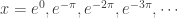
We consider the actual size of the negative powers of e and saw how they got exponentially smaller.
We did a practical problem in scaling to illustrate how fast the numbers diminish.

Why do I like this function?

What’s not to like?

Update (February 7, 2015) Chip Rollinson made this cool Geogebra applet to illustrate My Favorite Function. Use the slider on the screen and notice the x-axis scale as it changes. Thank you, Chip.

Students first encounter logarithms in Algebra 2 or their last pre-calculus course. They are usually defined as exponents and their properties “proven” by reference to the corresponding properties of exponents. This is good enough at the time, but in calculus we are ready to define logarithms properly. The result is the definition in terms of a function defined by an integral.

In fact, the definition flows naturally from the properties of inverse functions (no pun intended, because the flow is quite natural). But is this a definition? Or a proof? The solution of certain differential equations discussed in my last post may be used to derive the logarithm function.

Let’s begin by pretending we know nothing about logarithms, and investigate the inverse of e^x. (See The Derivative of Exponential Functions)

This function e^x contains points of the form $\left( X,{{e}^{X}} \right)$ so its inverse will contain points of the form $\left( {{e}^{X}},X \right)$ , which, since we like the first coordinate of functions to be x, we may also call $\left( x,\ln \left( x \right) \right)$ , where ln(x) will be the name of the inverse of e^x. Remember, at the moment ln(x) is just a notation for the inverse of e^x, we do not know anything about logarithms (yet).

So $\left( {{e}^{X}},X \right)$ = $\left( x,\ln \left( x \right) \right)$ and $X\ne x$ . For example, (0, 1) is a point on e^X, so (1, 0) is a point on the ln(x) function, and so ln(1) = 0.

In a previous post we defined the number e and the function e^x in such a way that $\displaystyle \frac{d}{dx}{{e}^{x}}={{e}^{x}}$ . Now, at $\left( X,{{e}^{X}} \right)$ the derivative is e^X, so at the corresponding point on its inverse, $\left( {{e}^{X}},X \right)$ , the derivative is the reciprocal of the derivative of e^X which is $\frac{1}{{{e}^{X}}}=\frac{1}{x}$ . That is

$\displaystyle \frac{d}{dx}\ln \left( x \right)=\frac{1}{x}$

We can use this idea to define ln(x) as a function defined by an integral. Solving the differential equation by the method suggested in a recent post we get:

$\displaystyle \ln \left( x \right)=\ln \left( a \right)+\int_{a}^{x}{\frac{1}{t}dx}$

We can pick any positive number for a and a convenient one is the one we already found a = 1 where ln(1) = 0, so

$\displaystyle \ln \left( x \right)=\int_{1}^{x}{\frac{1}{t}dx},\quad x>0$

This then is the “official definition” of the natural logarithm function. The domain is x > 0 (the range of e^x) and the range is all real numbers (the domain of e^x).

Graphically, ln(x) is the area between the graph of $\displaystyle \frac{1}{t}$ and the t-axis between 1 and x. If $0<x<1$ , then $\ln \left( x \right)<0$ and if $x>1$ , $\ln \left( x \right)>0$ .

From this definition we can prove all the familiar properties of logarithms $\left( \ln \left( ab \right)=\ln \left( a \right)+\ln \left( b \right)\text{ etc}\text{.} \right)$ and show that this is a function of the kind we called “logarithm” all along. This is in all the textbooks so I will not go into this here.

One of these properties tells us that for $a>0\text{ and }a\ne 1$ , $\displaystyle {{\log }_{a}}\left( x \right)=\frac{\ln \left( x \right)}{\ln \left( a \right)}$ and since ln(a) is a constant

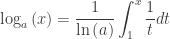
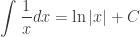$\displaystyle {{\log }_{a}}\left( x \right)=\frac{1}{\ln \left( a \right)}\int_{1}^{x}{\frac{1}{t}dt}$

Finally, you will see this antiderivative formula: $\displaystyle \int_{{}}^{{}}{\frac{1}{x}dx=\ln \left| x \right|+C}$ . The absolute value sign is to remind you that the argument of the logarithm function must be positive, since in some situations x itself may be negative.

Revised slightly 8-28-2018

Teaching Calculus

The pleasure lies not in discovering the truth, but in searching for it.

Tag Archives: exponential function

My Favorite Function

Logarithms

Share this:

Like this:

Share this:

Like this: