Variations on a Theme – 2

This is the second in an occasional series on adapting and expanding AP calculus exam questions. Variations on multiple-choice questions may make other multiple-choice questions, or, if you do not like making up all the “wrong” choices they can be changed to short answer questions for use in your class homework or test. Other variations make for good discussion questions.

 Today we will take a look at 2008 AB 10. This question gave the graph below and asked which of \displaystyle \int_{1}^{3}{f\left( x \right)dx}, a left, right, or midpoint Riemann sum approximation, or a trapezoidal sum approximation of the integral all with four subintervals of equal length has the least value.

Variations 2 pix 1

I’ll refer to these as I, L, R, M and T. The answer is R as a quick sketch will show.

In the discussion we will assume the curve does not change direction or concavity over the interval of integration. The answers to the questions in the variations are at the end of this post.

Variation 1: The question seems pretty easy so let’s beef it up a bit. How about asking the student to put I, L, R, M and T in order from smallest to largest? For a multiple-choice question answer choices are inequalities with all 5 sums in them.

The midpoint Riemann sum may be the most difficult to see. Here is the way to explain it. See the figure below.

Variations 2 pix 2

On each subinterval draw the horizontal segment at the function value at the midpoint of the interval. At this same point draw a tangent segment from one side of the interval to the other. This forms two congruent triangles with the horizontal segment and the edges of the interval.

Therefore, this midpoint trapezoid and the midpoint rectangle have the same area. Then because of the concavity, we see that in this case the midpoint Riemann sum, M, will be larger than the integral, I. With the same concavity the trapezoidal approximation will lie below the curve and therefore T < I < M. This will be true for any curve that is concave down. The opposite is true for a curve that is concave up: M < I < T. M and T are always on opposite sides of I. 

Variation 2: Change the number of subintervals, but keep the same number for each sum. Does this change anything?

Variation 3: Change the number of subintervals so that the sums over the same interval have a different number of subintervals. Does this change anything?

Variation 4: Change the shape of the curve to one of the other 4 shapes that a curve may have. How does this change the order of the sums?

Variation 5: Move the graph from above the ­x-axis to below. Does this change anything?

Variation 6: The reversal problem. Suppose that L < T < I < M < R; describe the shape of the curve. Other orders can be used as well. In fact this idea has appeared on an AP calculus exams. In 2003 AB 85 students were told that a trapezoidal sum over approximates and a right Riemann sum under approximates a certain integral. The question asked which of 5 graphs could be the graph of the function.

___________________

If you have other variations please click “Leave a Comment” to share them. If you have variations on a different question please share them as well.

___________________

Answers:

Variation 1: R < T < I < M < L

Variation 2: No. Since the order will be the same on each subinterval adding them will not change the order.

Variation 3: This makes a difference. In the first figure above, consider a trapezoidal sum with one subinterval compared to a right Riemann sum with many subintervals. The right Riemann sum will be very close to the integral with its rectangles ending above the trapezoidal segment between the endpoints. In this case T < R for the figure shown.

Variation 4: The left and right Riemann sums depend on whether the curve is decreasing or increasing. The Trapezoidal sum and the midpoint Riemann sum depend on the concavity. For example, an increasing concave up curve the order is L < M < I < T < R.

Variation 5: No. If the curve is entirely below the x-axis all the values will be negative, but all the results discussed in the other variations will be the same; the order will not change.

Variation 6: The curve is increasing and concave down.

Why Muss with the “+C”?

Here is a way to find the particular solution of a separable differential equation without using the +C and it might even be a little faster. As an example consider the initial value problem

\displaystyle \frac{dy}{dx}=\frac{y-1}{{{x}^{2}}}\text{ with }x\ne 0\text{ and }y\left( 2 \right)=0

Separate the variables as usual and then write each side a definite integral with the lower limit of integration the number from the initial condition and the upper limit variable. I’ll replace the dummy variable in the integrand with an upper-case X or Y to avoid having x and y in two places.

\displaystyle \int_{0}^{y}{\frac{1}{Y-1}dY}=\int_{2}^{x}{{{X}^{-2}}dX}

Integrate

\displaystyle \left. \ln \left| Y-1 \right| \right|_{0}^{y}=\left. -{{X}^{-1}} \right|_{2}^{x}

\displaystyle \ln \left| y-1 \right|-\ln \left| 0-1 \right|=-\frac{1}{x}+\frac{1}{2}

Note that near the initial condition where y = 0, \left( y-1 \right)<0 so \left| y-1 \right|=-\left( y-1 \right)=1-y . Continue and solve for y.

\displaystyle {{e}^{\ln \left( 1-y \right)}}={{e}^{-\frac{1}{x}+\frac{1}{2}}}

\displaystyle 1-y={{e}^{-\frac{1}{x}+\frac{1}{2}}}

\displaystyle y=1-{{e}^{-\frac{1}{x}+\frac{1}{2}}},\quad x>0

No muss; no fuss.


Variations on a Theme by ETS

Experienced AP calculus teacher use as many released exam questions during the year as they can. They are good questions and using them gets the students used to the AP style and format.  They can be used “as is”, but many are so rich that they can be tweaked to test other concepts and to make the students think wider and deeper.  

Below is a multiple-choice question from the 2008 AB calculus exam, question 9.

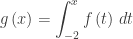
 2008 mc9The graph of the piecewise linear function f  is shown in the figure above. If \displaystyle g\left( x \right)=\int_{-2}^{x}{f\left( t \right)\,dt}, which of the following values is the greatest?

(A)  g(-3)         (B)  g(-2)         (C)  g(0)         (D)  g(1)         (E)  g(2)

I am now going to suggest some ways to tweak this question to bring out other ideas. Here are my suggestions. Some could be multiple-choice others simple short constructed response questions. A few of these questions, such as 3 and 4, ask the same thing in different ways.

      1. Require students to show work or justify their answer even on multiple-choice questions. So for this question they should write, “The answer is (D) g(1) since x = 1 is the only place where {g}'\left( x \right)=f\left( x \right) changes from positive to negative.” 
      2. Ask, “Which of the following values is the least?” (Same choices)
      3. Find the five values listed.
      4. Put the five values in order from smallest to largest.
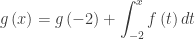
      5. If \displaystyle g\left( x \right)=g\left( -2 \right)+\int_{-2}^{x}{f\left( t \right)dt} and the maximum value of g is 7, what is the minimum value?
      6. If \displaystyle g\left( x \right)=g\left( -2 \right)+\int_{-2}^{x}{f\left( t \right)dt} and the minimum value of g is 7, what is the maximum value?
      7. Pick any number (not just an integers) in the interval [–3, 2] to be a and change the stem to read, “If \displaystyle g\left( x \right)=g\left( a \right)+\int_{a}^{x}{f\left( t \right)dt} ….” And then ask any of the questions above – some answers will be different, some will be the same. Discussing which will not change and why makes a worthwhile discussion.
      8. Change the equation in the stem to \displaystyle g\left( x \right)=3x+\int_{-2}^{x}{f\left( t \right)dt} and ask the questions above. Again most of the answers will change. Also this question and the next start looking like some free-response questions. Compare them with 2011 AB 4 and 2010 AB 5(c)
      9. Change the equation in the stem to \displaystyle g\left( x \right)=-\tfrac{3}{2}x+\int_{-2}^{x}{f\left( t \right)dt} and ask the questions above. This time most of the answers will change.
      10. Change the graph and ask the same questions.

Not all questions offer as many variations as this one. For some about all you can do is use them “as is” or just change the numbers.

Any other adaptations you can think of?

What is your favorite question for tweaking?

 Math in the News Combinatorics and UPS

Revised: August 24, 2014

Difficult Problems and Why We Like Them

Item 1:

Audrey Weeks writes a really great set of animations for calculus teachers and students called Calculus in Motion. The animations run on Geometer’s Sketchpad and are very easy to use, but difficult to program. But Audrey is an expert.  She is very busy each year at this time doing animations of the recent AP calculus exam questions. I proofread the animations as she finishes each one and now and then make some suggestions.

The particular solution to the differential equation question BC 5 on this year’s exam is a function with a vertical asymptote.  The animation allows the user to move the initial condition around. This moves the asymptote(s); in some cases there is no asymptote. Her graph showed the function on both sides of the asymptote with the note that the domain was x > –1.  I pointed out that the graph should only exist on one side of the asymptote at x = –1.  She wrote back that “I agree, and I had tried, but couldn’t find any way to do that.”  

Then the next day she sent the next version with only the correct part of the graph showing, and its changing restricted domain stated as the initial condition changed.

See the figure below with no graph to the left of the asymptote x = –1

cim

She wrote:

“Now, will anyone appreciate the additional 5 hours of work to make that happen, …?  Doesn’t matter … it makes ME happy.”

Item 2:

Kryptos is a sculpture by artist Jim Sanborn that stands on the campus of the Central Intelligence Agency (CIA) Headquarters in Langley,  VA.  The sculpture contains four coded messages.

Kryptos

In a recent article Wired.com recounts how David Stein, a CIA employee who is not a cryptographer, got interested in the cipher and spent 400 hours over 8 years trying to break it. He succeeded in deciphering three of the four messages in 1998. He did the deciphering with pencil-and-paper in his spare time.

The CIA would not allow him to make his results public at the time.  (Later, Jim Gillogly, a computer scientist, cracked the same 3 messages using a computer and, not being employed by the CIA, published his results.)  The CIA recently declassified Stein work.

The Wired article recounts the story when (quoting Stein), “I was I was hit by that sweetly ecstatic, rare experience that I have heard described as a ‘moment of clarity.’ All the doubts and speculations about the thousands of possible alternate paths simply melted away, and I clearly saw the one correct course laid out in front of me.”  Stein’s full article is included in the Wired article (photocopied, slightly redacted, and missing the figures and charts). The solution is here. To this day no one has deciphered the fourth message.

Stein’s account concludes with this remark:

When confronted with a puzzle or problem, we sometimes can lose sight of the fact that we have issued a challenge to ourselves–not to our tools. And before we automatically reach for our computers, we sometimes need to remember that we already possess the most essential and powerful problem-solving tool within our own minds.

In other words, he did it because it made him happy.

Photo by Jim Sanborn – Wikipedia

Update (November 21, 2014) The sculptor of Kryptos has provide a second clue to the fourth panel of the sculptor. The full story is here. The full enciphered text is below. The source (N.Y. Times November 21, 2014) with the known deciphering and the clues is here.

kryptos-945

L’Hôpital Rules the Graph

In my last post on May 31, 2012 I showed a way of demonstrating why L’Hôpital’s Rule works. We looked at an example,

\displaystyle \underset{x\to \pi }{\mathop{\lim }}\,\frac{\tan \left( x \right)}{\sin \left( x \right)},

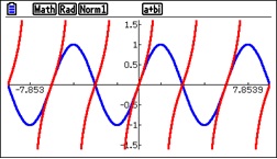
which met the requirement of the theorem called L’Hôpital’s Rule, namely the functions are differentiable and, since  tan(\pi ) = sin(\pi ) = 0 they intersect on the x-axis at \left( \pi ,0 \right). We looked at the graph and then zoomed-in at \left( \pi ,0 \right).
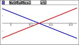
L’Hôpital’s Rule tells us that with these conditions the limit is the same as the limit of the ratio of their slopes (or their derivatives, if you prefer). Can you see what that ratio is from Figure 2? Even though this is not a “square window” the ratio is obviously –1.

Here are four other limits. See if you can find them by the method suggested here. Namely zoom-in on the point where the functions intersect and see if you can find the limits without doing any computations. (Yes, I know you already know the first 3, but try this idea anyway. )

1. \displaystyle \underset{x\to 0}{\mathop{\lim }}\,\frac{\sin \left( x \right)}{x}

2. \displaystyle \underset{x\to 0}{\mathop{\lim }}\,\frac{1-\cos \left( x \right)}{x}

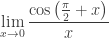
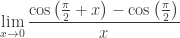
3. \displaystyle \underset{x\to 0}{\mathop{\lim }}\,\frac{\cos \left( \tfrac{\pi }{2}+x \right)}{x} also known as \displaystyle \underset{x\to 0}{\mathop{\lim }}\,\frac{\cos \left( \tfrac{\pi }{2}+x \right)-\cos \left( \tfrac{\pi }{2} \right)}{x}

4. \displaystyle \underset{x\to 1}{\mathop{\lim }}\,\frac{\pi \ln \left( x \right)}{\sin \left( \pi x \right)}


Answers in order:  1, 0, -1, -1

Locally Linear L’Hôpital

I’ll begin with a lemma. (I like to do a lemma now and then if for no other reason than having an excuse to explain what a lemma is – a simple theorem that is used in proving the main theorem.)

Lemma: If two lines intersect on the x-axis, then for any x the ratio of their y-coordinates is equal to the ratio of their slopes.

Proof: Two lines with slopes of m1 and m2 that intersect at (a, 0) on the x-axis have equations y1 = m1(xa) and y2 = m2(xa). Then

\displaystyle \frac{{{y}_{1}}}{{{y}_{2}}}=\frac{{{m}_{1}}\left( x-a \right)}{{{m}_{2}}\left( x-a \right)}=\frac{{{m}_{1}}}{{{m}_{2}}}

L’Hôpital’s Rule (Theorem): If f and g are differentiable near x = a and f(a) = g(a) = 0, then

\displaystyle \underset{x\to a}{\mathop{\lim }}\,\frac{f\left( x \right)}{g\left( x \right)}=\underset{x\to a}{\mathop{\lim }}\,\frac{{f}'\left( x \right)}{{g}'\left( x \right)}

if the limit exists.

The fact that f(a) = g(a) = 0 means that the two functions intersect on the x-axis at (a, 0). For example, the functions f(x) = tan(x) and g(x) = sin(x) have this property at \left( \pi ,0 \right).

Figure 1. y = tan(x) in red and y = sin(x) in blue

Figure 1. y = tan(x) in red and y = sin(x) in blue

Now zoom-in several times centered at \left( \pi ,0 \right).

Figure 2. The previous graph zoomed in.

Figure 2. The previous graph zoomed in.

Whoa!

That looks like lines!!

It’s the local linearity property of differentiable functions – if you zoom-in enough any differentiable function eventually looks linear. So maybe near \left( \pi ,0 \right) the lemma applies. The only difference is that the slopes of the “lines” are the derivatives so

\displaystyle \underset{x\to a}{\mathop{\lim }}\,\frac{f\left( x \right)}{g\left( x \right)}=\underset{x\to a}{\mathop{\lim }}\,\frac{{f}'\left( x \right)}{{g}'\left( x \right)}

 Now that does not quite prove L’Hôpital’s Rule, but it should give you and your students a good idea of why L’Hôpital’s Rule is true.

Then in our example:

\displaystyle \underset{x\to \pi }{\mathop{\lim }}\,\frac{\tan \left( x \right)}{\sin \left( x \right)}=\underset{x\to \pi }{\mathop{\lim }}\,\frac{\frac{1}{{{\left( \cos \left( x \right) \right)}^{2}}}}{\cos \left( x \right)}=\underset{x\to \pi }{\mathop{\lim }}\,\frac{1}{{{\left( \cos \left( x \right) \right)}^{3}}}=\frac{1}{{{\left( \cos \left( \pi \right) \right)}^{3}}}=-1

But isn’t that obvious from Figure 2?

Think about it.

More on this next time.


Summer Reading

I like to read and I read a lot. I often have a novel going. Lately since I’ve been writing this Blog, I’ve been reading other blogs. I’ve listed a few in the right-side column but here are two that might interest you. (Since deleted)

Wired Magazine

Wired magazine  has a lot of interesting articles on science and technology. They also publish a collection of Science Blogs. If you are interested in what’s going on in science this may be the place to start. Samuel Arbesman writes the math blog entitled Social Dimensions that is more focused on things mathematical. Wired also has the latest in math news like their piece on the “Unknown Mathematician Proves Elusive Property of Prime Numbers”

 dy/dan

Another of my favorites is a blog called dy/dan  by Dan Meyer who always has interesting ideas and interesting problems to discuss from all levels of teaching mathematics. The blog has lessons on lots of topics.

Dan recently posted the video below. It is a talk by Uri Theisman entitled “Keeping Our Eyes on the Prize” concerning equity, race and the opportunity to learn. Dr. Theisman is from the Charles A. Dana Center at the University of Texas at Austin. He is a recognized authority on education. The talk was given at the NCTM meeting April 19, 2103. It runs about 50 minutes and is certainly worth the time. Anyone interested in equity and the opportunity to learn will find this interesting.  Here is Dr. Theisman’s own summary:

There are two factors that shape inequality in this country and educational achievement inequality. The big one is poverty. But a really big one is an opportunity to learn. As citizens, we need to work on poverty and income inequality or our democracy is threatened. As mathematics educators … we need to work on opportunity to learn. It cannot be that the accident of where a child lives or the particulars of their birth determine their mathematics education.

Uri Treisman’s “Keeping Our Eyes on the Prize” – NCTM 2013 from Dan Meyer on Vimeo.

Is God a Mathematician?

Finally, if you are looking for an actual book to read, I recommend again Is God a Mathematician? by Mario Livio. I written about this book before here.