Area and Volume Problems (Type 4)

Posted on March 13, 2020 by Lin McMullin

AP Type Questions 4: Area and Volume

Given equations that define a region in the plane students are asked to find its area, the volume of the solid formed when the region is revolved around a line, and/or the region is used as a base of a solid with regular cross-sections. This standard application of the integral has appeared every year since year one (1969) on the AB exam and almost every year on the BC exam. You can be pretty sure that if a free-response question on areas and volumes does not appear, the topic will be tested on the multiple-choice section.

What students should be able to do:

Find the intersection(s) of the graphs and use them as limits of integration (calculator equation solving). Write the equation followed by the solution; showing work is not required. Usually no credit is earned until the solution is used in context (as a limit of integration). Students should know how to store and recall these values to save time and avoid copy errors.
Find the area of the region between the graph and the x-axis or between two graphs.
Find the volume when the region is revolved around a line, not necessarily an axis or an edge of the region, by the disk/washer method. See “Subtract the Hole from the Whole”
The cylindrical shell method will never be necessary for a question on the AP exams, but is eligible for full credit if properly used.
Find the volume of a solid with regular cross-sections whose base is the region between the curves. For an interesting variation on this idea see 2009 AB 4(b)
Find the equation of a vertical line that divides the region in half (area or volume). This involves setting up an integral equation where the limit is the variable for which the equation is solved.
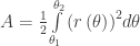
For BC only – find the area of a region bounded by polar curves: $A=\tfrac{1}{2}\int\limits_{{{\theta }_{1}}}^{{{\theta }_{2}}}{{{\left( r\left( \theta \right) \right)}^{2}}}d\theta$
For BC only – Find perimeter using arc length integral

If this question appears on the calculator active section, it is expected that the definite integrals will be evaluated on a calculator. Students should write the definite integral with limits on their paper and put its value after it. It is not required to give the antiderivative and if a student gives an incorrect antiderivative they will lose credit even if the final answer is (somehow) correct.

There is a calculator program available that will give the set-up and not just the answer so recently this question has been on the no calculator allowed section. (The good news is that in this case the integrals will be easy or they will be set-up-but-do-not-integrate questions.)

Occasionally, other type questions have been included as a part of this question. See 2016 AB5/BC5 which included an average value question and a related rate question along with finding the volume.

Shorter questions on this concept appear in the multiple-choice sections. As always, look over as many questions of this kind from past exams as you can find.

For some previous posts on this subject see January 9, 11, 2013 and “Subtract the Hole from the Whole” of December 6, 2016.

The Area and Volume question covers topics from Unit 6 of the 2019 CED .

Free-response questions:

Variations: 2009 AB 4, Don’t overlook this one, especially part (b)
2016 AB5/BC5,
2017 AB 1 (using a table),
2018 AB 5 – average rate of change, L’Hospital’s Rule
2019 AB 5
Perimeter parametric curves 2011 BC 3 and 2014 BC 5
Area in polar form 2017 BC 5, 2018 BC 5, 20129 BC 2

Multiple-choice questions from non-secure exams:

2008 AB 83 (Use absolute value),
2012 AB 10, 92
2012 BC 87, 92 (Polar area)

Revised March 12, 2012

Graph Analysis Questions (Type 3)

Posted on March 10, 2020 by Lin McMullin

AP Questions Type 3: Graph Analysis

The long name is “Here’s the graph of the derivative, tell me things about the function.”

Students are given either the equation of the derivative of a function or a graph identified as the derivative of a function with no equation is given. It is not expected that students will write the equation of the function from the graph (although this may be possible); rather, students are expected to determine important features of the function directly from the graph of the derivative. They may be asked for the location of extreme values, intervals where the function is increasing or decreasing, concavity, etc. They may be asked for function values at points. They will be asked to justify their conclusions.

The graph may be given in context and student will be asked about that context. The graph may be identified as the velocity of a moving object and questions will be asked about the motion. See Linear Motion Problems (Type 2)

Less often the function’s graph may be given and students will be asked about its derivatives.

What students should be able to do:

Read information about the function from the graph of the derivative. This may be approached by derivative techniques or by antiderivative techniques.
Find and justify where the function is increasing or decreasing.
Find and justify extreme values (1^st and 2^nd derivative tests, Closed interval test a/k/a Candidates’ test).
Find and justify points of inflection.
Find slopes (second derivatives, acceleration) from the graph.
Write an equation of a tangent line.
Evaluate Riemann sums from geometry of the graph only. This usually involves familiar shapes such as triangles or semicircles.
FTC: Evaluate integral from the area of regions on the graph.
FTC: The function, g(x), maybe defined by an integral where the given graph is the graph of the integrand, f(t), so students should know that if,

$\displaystyle g\left( x \right)=g\left( a \right)+\int_{a}^{t}{f\left( t \right)dt}$ then ${g}'\left( x \right)=f\left( x \right)$ and ${{g}'}'\left( x \right)={f}'\left( x \right)$ .

In this case, students should write ${g}'(t)=f\left( t \right)$ on their answer paper, so it is clear to the reader that they understand this.

Not only must students be able to identify these things, but they are usually asked to justify their answer and reasoning. See Writing on the AP Exams for more on justifying and explaining answers.

The ideas and concepts that can be tested with this type question are numerous. The type appears on the multiple-choice exams as well as the free-response. Between multiple-choice and free-response this topic may account for 15% or more of the points available on recent tests. It is very important that students are familiar with all the ins and outs of this situation.

As with other questions, the topics tested come from the entire year’s work, not just a single unit. In my opinion many textbooks do not do a good job with integrating these topics, so be sure to use as many actual AP Exam questions as possible. Study past exams; look them over and see the different things that can be asked. The Graph Analysis problem may cover topics primarily from primarily from Unit 4, Unit 5, and Unit 8 of the 2019 CED

For some previous posts on this subject see October 15, 17, 19, 24, 26 (my most read post), 2012 and January 25, 28, 2013

Free-response questions:

Function given as a graph, questions about its integral (so by FTC the graph is the derivative): 2016 AB 3/BC 3, 2018 AB3
Table and graph of function given, questions about related functions: 2017 AB 6,
Derivative given as a graph: 2016 AB 3 and 2017 AB 3
Information given in a table 2014 AB 5

Multiple-choice questions from non-secure exam. Notice the number of questions all from the same year; this is in addition to one free-response question (~25 points on AB and ~23 points on BC out of 108 points total)

2012 AB: 2, 5, 15, 17, 21, 22, 24, 26, 76, 78, 80, 83, 82, 84, 85, 87
2012 BC 3, 11, 12, 15, 12, 18, 21, 76, 78, 80, 81, 84, 88, 89

A good activity on this topic is here. The first pages are the teacher’s copy and solution. Then there are copies for Groups A, B, and C. Divide your class into 3 or 6 or 9 groups and give one copy to each. After they complete their activity have the students compare their results with the other groups.

Revised March 12, 2021

Linear Motion (Type 2)

Posted on March 6, 2020 by Lin McMullin

AP Questions Type 2: Linear Motion

We continue the discussion of the various type questions on the AP Calculus Exams with linear motion questions.

“A particle (or car, person, or bicycle) moves on a number line ….”

These questions may give the position equation, the velocity equation (most often), or the acceleration equation of something that is moving on the x– or y-axis as a function of time, along with an initial condition. The questions ask for information about motion of the particle: its direction, when it changes direction, its maximum position in one direction (farthest left or right), its speed, etc.

The particle may be a “particle,” a person, car, a rocket, etc. Particles don’t really move in this way, so the equation or graph should be considered to be a model. The question is a versatile way to test a variety of calculus concepts since the position, velocity, or acceleration may be given as an equation, a graph, or a table; be sure to use examples of all three forms during the review.

Many of the concepts related to motion problems are the same as those related to function and graph analysis (Type 3). Stress the similarities and show students how the same concepts go by different names. For example, finding when a particle is “farthest right” is the same as finding the when a function reaches its “absolute maximum value.” See my post for Motion Problems: Same Thing, Different Context for a list of these corresponding terms. There is usually one free-response question and three or more multiple-choice questions on this topic.

The position, s(t), is a function of time. The relationships are:

The velocity is the derivative of the position, ${s}'\left( t \right)=v\left( t \right)$ . Velocity is has direction (indicated by its sign) and magnitude. Technically, velocity is a vector; the term “vector” will not appear on the AB exam.
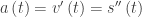Speed is the absolute value of velocity; it is a number, not a vector. See my post for Speed.
Acceleration is the derivative of velocity and the second derivative of position, $\displaystyle a\left( t \right)={v}'\left( t \right)={{s}''}\left( t \right)$ . It, too, has direction and magnitude and is a vector.
Velocity is the antiderivative of the acceleration.
Position is the antiderivative of velocity.

What students should be able to do:

Understand and use the relationships above.
Distinguish between position at some time and the total distance traveled during the time period.
The total distance traveled is the definite integral of the speed (absolute value of velocity) $\displaystyle \int_{a}^{b}{\left| v\left( t \right) \right|}\,dt$ .
Be sure your students understand the term displacement; it is the net distance traveled or distance between the initial position and the final position. Displacement, is the definite integral of the velocity (rate of change): $\displaystyle \int_{a}^{b}{v\left( t \right)}\,dt$ .
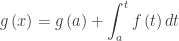
The final position is the initial position plus the displacement (definite integral of the rate of change from x= a to x = t): $\displaystyle s\left( t \right)=s\left( a \right)+\int_{a}^{t}{v\left( x \right)}\,dx$ Notice that this is an accumulation function equation (Type 1).
Initial value differential equation problems: given the velocity or acceleration with initial condition(s) find the position or velocity. These are easily handled with the accumulation equation in the bullet above, but may also be handled as an initial value problem.
Find the speed at a given time. The speed is the absolute value of the velocity.
Find average speed, velocity, or acceleration
Determine if the speed is increasing or decreasing.
- If at some time, the velocity and acceleration have the same sign then the speed is increasing.If they have different signs the speed is decreasing.
- If the velocity graph is moving away from (towards) the t-axis the speed is increasing (decreasing). See the post on Speed.
- There is also a worksheet on speed here
- The analytic approach to speed: A Note on Speed
Use a difference quotient to approximate the derivative (velocity or acceleration) from a table. Be sure the work shows a quotient.
Riemann sum approximations.
Units of measure.
Interpret meaning of a derivative or a definite integral in context of the problem

Shorter questions on this concept appear in the multiple-choice sections. As always, look over as many questions of this kind from past exams as you can find.

This may be an AB or BC question. The BC topic of motion in a plane, (Type 8: parametric equations and vectors) will be discussed in a later post.

The Linear Motion problem may cover topics primarily from primarily from Unit 4, and also from Unit 3, Unit 5, Unit 6, and Unit 8 (for BC) of the 2019 CED.

Free-response examples:

Equation stem 2017 AB 5,
Graph stem: 2009 AB1/BC1,
Table stem 2019 AB2

Multiple-choice examples from non-secure exams:

2012 AB 6, 16, 28, 79, 83, 89
2012 BC 2, 89

Rate & Accumulation (Type 1)

Posted on March 3, 2020 by Lin McMullin

The Free-response Questions

There are ten general categories of AP Calculus free-response questions.

NOTE: The type number I’ve assigned to each type DO NOT correspond to the 2019 CED Unit numbers. Many AP Exam questions have parts from different Units. The CED Unit numbers will be referenced in each post.

AP Questions Type 1: Rate and Accumulation

These questions are often in context with a lot of words describing a situation in which some things are changing. There are usually two rates acting in opposite ways (sometimes called an in-out question). Students are asked about the change that the rates produce over some time interval either separately or together.

The rates are often fairly complicated functions. If they are on the calculator allowed section, students should store the functions in the equation editor of their calculator and use their calculator to do any graphing, integration, or differentiation that may be necessary.

The main idea is that over the time interval [a, b] the integral of a rate of change is the net amount of change

$\displaystyle \int_{a}^{b}{{f}'\left( t \right)dt}=f\left( b \right)-f\left( a \right)$

If the question asks for an amount, look around for a rate to integrate.

The final (accumulated) amount is the initial amount plus the accumulated change:

$\displaystyle f\left( x \right)=f\left( {{x}_{0}} \right)+\int_{{{x}_{0}}}^{x}{{f}'\left( t \right)}\,dt$ ,

where ${{x}_{0}}$ is the initial time, and $f\left( {{x}_{0}} \right)$ is the initial amount. Since this is one of the main interpretations of the definite integral the concept may come up in a variety of situations.

What students should be able to do:

Be ready to read and apply; often these problems contain a lot of writing which needs to be carefully read.
Recognize that rate = derivative.
Recognize a rate from the units given without the words “rate” or “derivative.”
Find the change in an amount by integrating the rate. The integral of a rate of change gives the amount of change (FTC):

$\displaystyle \int_{a}^{b}{{f}'\left( t \right)dt}=f\left( b \right)-f\left( a \right)$ .

Find the final amount by adding the initial amount to the amount found by integrating the rate. If $x={{x}_{0}}$ is the initial time, and $f\left( {{x}_{0}} \right)$ is the initial amount, then final accumulated amount is

$\displaystyle f\left( x \right)=f\left( {{x}_{0}} \right)+\int_{{{x}_{0}}}^{x}{{f}'\left( t \right)}\,dt$ ,

Write an integral expression that gives the amount at a general time. BE CAREFUL, the dt must be included at the correct place. Think of the integral sign and the dt as parentheses around the integrand.
Find the average value of a function
Understand the question. It is often not necessary to as much computation as it seems at first.
Use FTC to differentiate a function defined by an integral.
Explain the meaning of a derivative or its value in terms of the context of the problem. The explanation should contain (1) what it represents, (2) its units, and (3) how numerical argument applies in context.
Explain the meaning of a definite integral or its value in terms of the context of the problem. The explanation should contain (1) what it represents, (2) its units, and (3) how the limits of integration apply in context.
Store functions in their calculator recall them to do computations on their calculator.
If the rates are given in a table, be ready to approximate an integral using a Riemann sum or by trapezoids.
Do a max/min or increasing/decreasing analysis.

Shorter questions on this concept appear in the multiple-choice sections. As always, look over as many questions of this kind from past exams as you can find.

The Rate – Accumulation question may cover topics primarily from Unit 4, Unit 5, Unit 6 and Unit 8 of the 2019 CED.

Typical free-response examples:

2013 AB1/BC1
2015 AB1/BC1
2018 AB1/BC1
2019 AB1/BC1
One of my favorites Good Question 6 (2002 AB 4)

Typical multiple-choice examples from non-secure exams:

2012 AB 8, 81, 89
2012 BC 8 (same as AB 8)

Updated January 31, 2019, March 12, 2021

2019 CED Unit 8: Applications of Integration

Posted on December 3, 2019 by Lin McMullin

This unit seems to fit more logically after the opening unit on integration (Unit 6). The Course and Exam Description (CED) places Unit 7 Differential Equations before Unit 8 probably because the previous unit ended with techniques of antidifferentiation. My guess is that many teachers will teach Unit 8: Applications of Integration immediately after Unit 6 and before Unit 7: Differential Equations. The order is up to you.

Unit 8 includes some standard problems solvable by integration (CED – 2019 p. 143 – 161). These topics account for about 10 – 15% of questions on the AB exam and 6 – 9% of the BC questions.

Topics 8.1 – 8.3 Average Value and Accumulation

Topic 8.1 Finding the Average Value of a Function on an Interval Be sure to distinguish between average value of a function on an interval, average rate of change on an interval and the mean value

Topic 8.2 Connecting Position, Velocity, and Acceleration of Functions using Integrals Distinguish between displacement (= integral of velocity) and total distance traveled (= integral of speed)

Topic 8. 3 Using Accumulation Functions and Definite Integrals in Applied Contexts The integral of a rate of change equals the net amount of change. A really big idea and one that is tested on all the exams. So, if you are asked for an amount, look around for a rate to integrate.

Topics 8.4 – 8.6 Area

Topic 8.4 Finding the Area Between Curves Expressed as Functions of x

Topic 8.5 Finding the Area Between Curves Expressed as Functions of y

Topic 8.6 Finding the Area Between Curves That Intersect at More Than Two Points Use two or more integrals or integrate the absolute value of the difference of the two functions. The latter is especially useful when do the computation of a graphing calculator.

Topics 8.7 – 8.12 Volume

Topic 8.7 Volumes with Cross Sections: Squares and Rectangles

Topic 8.8 Volumes with Cross Sections: Triangles and Semicircles

Topic 8.9 Volume with Disk Method: Revolving around the x– or y-Axis Volumes of revolution are volumes with circular cross sections, so this continues the previous two topics.

Topic 8.10 Volume with Disk Method: Revolving Around Other Axes

Topic 8.11 Volume with Washer Method: Revolving Around the x– or y-Axis See Subtract the Hole from the Whole for an easier way to remember how to do these problems.

Topic 8.12 Volume with Washer Method: Revolving Around Other Axes. See Subtract the Hole from the Whole for an easier way to remember how to do these problems.

Topic 8.13 Arc Length BC Only

Topic 8.13 The Arc Length of a Smooth, Planar Curve and Distance Traveled BC ONLY

Timing

The suggested time for Unit 8 is 19 – 20 classes for AB and 13 – 14 for BC of 40 – 50-minute class periods, this includes time for testing etc.

Previous posts on these topics for both AB and BC include:

Average Value and Accumulation

Average Value of a Function and Average Value of a Function

Half-full or Half-empty

Accumulation: Need an Amount?

AP Accumulation Questions

Good Question 7 – 2009 AB 3 Accumulation, explain the meaning of an integral in context, unit analysis

Good Question 8 – or Not Unit analysis

Graphing with Accumulation 1 Seeing increasing and decreasing through integration

Graphing with Accumulation 2 Seeing concavity through integration

Area

Area Between Curves

Under is a Long Way Down Avoiding “negative area.”

Improper Integrals and Proper Areas BC Topic

Math vs. the “Real World” Improper integrals BC Topic

Volume

Volumes of Solids with Regular Cross-sections

Volumes of Revolution

Why You Never Need Cylindrical Shells

Visualizing Solid Figures 1

Visualizing Solid Figures 2

Visualizing Solid Figures 3

Visualizing Solid Figures 4

Visualizing Solid Figures 5

Painting a Point

Subtract the Hole from the Whole and Does Simplifying Make Things Simpler?

Other Applications of Integrals

Density Functions have been tested in the past, but are not specifically listed on the CED then or now.

Who’d a Thunk It? Some integration problems suitable for graphing calculator solution

Here are links to the full list of posts discussing the ten units in the 2019 Course and Exam Description.

2019 CED – Unit 1: Limits and Continuity

2019 CED – Unit 2: Differentiation: Definition and Fundamental Properties.

2019 CED – Unit 3: Differentiation: Composite , Implicit, and Inverse Functions

2019 CED – Unit 4 Contextual Applications of the Derivative Consider teaching Unit 5 before Unit 4

2019 – CED Unit 5 Analytical Applications of Differentiation Consider teaching Unit 5 before Unit 4

2019 – CED Unit 6 Integration and Accumulation of Change

2019 – CED Unit 7 Differential Equations Consider teaching after Unit 8

2019 – CED Unit 8 Applications of Integration Consider teaching after Unit 6, before Unit 7

2019 – CED Unit 9 Parametric Equations, Polar Coordinates, and Vector-Values Functions

2019 CED Unit 10 Infinite Sequences and Series

2019 CED Unit 7: Differential Equations

Posted on November 26, 2019 by Lin McMullin

Applications (Unit 8) seem to fit more logically after the opening unit on integration (Unit 6). The Course and Exam Description (CED) present differential equations first probably because the previous unit ended with techniques of antidifferentiation. My guess is that many teachers will teach Unit 8: Applications of Integration before Unit 7: Differential Equations. Therefore, for those who want to present unit 8 first, I will post unit 8 next week on December 3, 2019. That way you’ll have both for reference and can choose the order you think will work best for your students.

Unit 7 is an introduction to the initial ideas and easy techniques related to differential equations. (CED – 2019 p. 129 – 142). These topics account for about 6 – 12% of questions on the AB exam and 6 – 9% of the BC questions.

Topics 7.1 – 7.9

Topic 7.1 Modeling Situations with Differential Equations Relating a function and its derivatives.

Topic 7.2 Verifying Solutions for Differential Equations A proposed solution to a differential equation can be checked by substituting the function and its derivative(s) into the original differential equation. There may be an infinite number of general solutions (solutions with one or more constants).

Topic 7.3 Sketching Slope Fields Slope fields are a graphical representation of a differential equation and provide information about the behavior of the solutions.

Topic 7.4 Reasoning Using Slope Fields

Topic 7.5 Approximating Solutions Using Euler’s method (BC ONLY) A numerical approach to approximating solutions of a differential equation.

Topic 7.6 Finding General Solutions Using Separation of Variable Since this unit is only an introduction to differential equations, the method of separation of variable is the only solution method tested on the AB and BC exams.

Topic 7.7 Finding Particular Solutions Using Initial Conditions and Separation of Variables An initial condition (i.e. a point on the particular solution) allows you to evaluate the constant in the general solution and find the one solution that contains the initial condition. Also, if $\displaystyle \frac{{dy}}{{dx}}=f\left( x \right)$ has the initial condition $\displaystyle \left( {a,F\left( a \right)} \right)$ , then the solution is $\displaystyle F\left( x \right)=F\left( a \right)+\int_{a}^{x}{{f\left( x \right)dx}}$ . Solution may also be subject to domain restrictions.

Topic 7.8 Exponential Models with Differential Equations Applications include linear motion and exponential growth and decay. The growth and decay model is $\displaystyle \frac{{dy}}{{dt}}=ky$ with the initial condition $\displaystyle (0,{{y}_{0}})$ has the solution $\displaystyle y={{y}_{0}}{{e}^{{kt}}}$ .

Topic 7.9 Logistic Models with Differential Equations (BC ONLY) The model of logistic growth, $\displaystyle \frac{{dy}}{{dt}}=ky\left( {a-y} \right)$ , can be solved by separating the variables and using partial fraction decomposition. This has never been tested (probably because solving requires a large amount of complicated algebra). Students are expected to know how to interpret the properties of the solution directly from the differential equation (asymptotes, carrying capacity, point where changing the fastest, etc.) and discuss what they mean in context without actually solving the equation.

Timing

The suggested time for Unit 7 is 8 – 9 classes for AB and 9 – 10 for BC of 40 – 50-minute class periods, this includes time for testing etc.

Previous posts on these topics for both AB and BC include:

Differential Equations A summary of the terms and techniques about differential equations and the method of separation of variables

Domain of a Differential Equation – On domain restrictions.

Accumulation and Differential Equations

Slope Fields

An Exploration in Differential Equations An exploration illustrating many of the ideas of differential equations. The exploration is here in PDF form and the solution is here. The ideas include: finding the general solution of the differential equation by separating the variables, checking the solution by substitution, using a graphing utility to explore the solutions for all values of the constant of integration, finding the solutions’ horizontal and vertical asymptotes, finding several particular solutions, finding the domains of the particular solutions, finding the extreme value of all solutions in terms of C, finding the second derivative (implicit differentiation), considering concavity, and investigating a special case or two.

Posts on BC Only Topics

Euler’s Method

Euler’s Method for Making Money

The Logistic Equation

Logistic Growth – Real and Simulated

Here are links to the full list of posts discussing the ten units in the 2019 Course and Exam Description.

2019 CED – Unit 1: Limits and Continuity

2019 CED – Unit 2: Differentiation: Definition and Fundamental Properties.

2019 CED – Unit 3: Differentiation: Composite , Implicit, and Inverse Functions

2019 CED – Unit 4 Contextual Applications of the Derivative Consider teaching Unit 5 before Unit 4

2019 – CED Unit 5 Analytical Applications of Differentiation Consider teaching Unit 5 before Unit 4

2019 – CED Unit 6 Integration and Accumulation of Change

2019 – CED Unit 7 Differential Equations Consider teaching after Unit 8

2019 – CED Unit 8 Applications of Integration Consider teaching after Unit 6, before Unit 7

2019 – CED Unit 9 Parametric Equations, Polar Coordinates, and Vector-Values Functions

2019 CED Unit 10 Infinite Sequences and Series

2019 CED Unit 6: Integration and Accumulation of Change

Posted on November 12, 2019 by Lin McMullin

Unit 6 develops the ideas behind integration, the Fundamental Theorem of Calculus, and Accumulation. (CED – 2019 p. 109 – 128 ). These topics account for about 17 – 20% of questions on the AB exam and 17 – 20% of the BC questions.

Topics 6.1 – 6.4 Working up to the FTC

Topic 6.1 Exploring Accumulations of Change Accumulation is introduced through finding the area between the graph of a function and the x-axis. Positive and negative rates of change, unit analysis.

Topic 6.2 Approximating Areas with Riemann Sums Left-, right-, midpoint Riemann sums, and Trapezoidal sums, with uniform partitions are developed. Approximating with numerical methods, including use of technology are considered. Determining if the approximation is an over- or under-approximation.

Topic 6.3 Riemann Sums, Summation Notation and the Definite Integral. The definition integral is defined as the limit of a Riemann sum.

Topic 6.4 The Fundamental Theorem of Calculus (FTC) and Accumulation Functions Functions defined by definite integrals and the FTC.

Topic 6.5 Interpreting the Behavior of Accumulation Functions Involving Area Graphical, numerical, analytical, and verbal representations.

Topic 6.6 Applying Properties of Definite Integrals Using the properties to ease evaluation, evaluating by geometry and dealing with discontinuities.

Topic 6.7 The Fundamental Theorem of Calculus and Definite Integrals Antiderivatives. (Note: I suggest writing the FTC in this form $\displaystyle \int_{a}^{b}{{{f}'\left( x \right)}}dx=f\left( b \right)-f\left( a \right)$ because it seems more efficient than using upper case and lower-case f.)

Topics 6.5 – 6.14 Techniques of Integration

Topic 6.8 Finding Antiderivatives and Indefinite Integrals: Basic Rules and Notation. Using basic differentiation formulas to find antiderivatives. Some functions do not have closed-form antiderivatives. (Note: While textbooks often consider antidifferentiation before any work with integration, this seems like the place to introduce them. After learning the FTC students have a reason to find antiderivatives. See Integration Itinerary

Topic 6.9 Integration Using Substitution The u-substitution method. Changing the limits of integration when substituting.

Topic 6.10 Integrating Functions Using Long Division and Completing the Square

Topic 6.11 Integrating Using Integration by Parts (BC ONLY)

Topic 6.12 Integrating Using Linear Partial Fractions (BC ONLY)

Topic 6.13 Evaluating Improper Integrals (BC ONLY) Showing the work requires students to show correct limit notation.

Topic 6.14 Selecting Techniques for Antidifferentiation This means practice, practice, practice.