Why the Fundamental Theorem of Calculus?

Posted on November 28, 2023 by Lin McMullin

The Fundamental Theorem of Calculus is, well, fundamental. It relates the derivative and the integral.

Writing a Riemann sum with all that fancy notation is tedious. To speed things up a special notation is used to replace it. The limit of the Riemann sum for a function on an interval [a, b] is written as its definite integral:

$\displaystyle \underset{{\left| {\Delta x} \right|\to 0}}{\mathop{{\lim }}}\,\sum\limits_{{i=1}}^{\infty }{{f\left( {{{x}_{i}}} \right)\Delta x}}$ $\displaystyle =\int_{a}^{b}{{f\left( x \right)dx}}$

The $\displaystyle f\left( x \right)$ (called the integrand) is the function with no fancy notation and the dx, called differential x replaces the $\displaystyle \Delta x$ . The a and b, called the lower and upper limit of integration respectively, show you the interval the Riemann sum was formed on (which the Riemann sum does not).

Keep in mind that behind every definite integral is a Riemann sum. Therefore, all the properties of limits apply to definite integrals. They can be added and subtracted, a constant may be factored out, and so on.

The Fundamental Theorem of Calculus, the FTC, tells you how to evaluate a definite integral (and therefore its Riemann sum): Simply evaluate the function of which $\displaystyle f\left( x \right)$ is the derivative at the endpoints of the interval and subtract.

To keep this in mind you can write the FTC like this considering the integrand as the derivative (of something):

$\displaystyle \int_{a}^{b}{{{f}'\left( x \right)dx}}=f\left( b \right)-f\left( a \right)$ .

For example, since $\displaystyle d\sin \left( x \right)=\cos \left( x \right)dx$ ,

$\displaystyle \int_{0}^{{\pi /2}}{{\cos \left( x \right)dx=\sin }}\left( {\tfrac{\pi }{2}} \right)-\sin \left( 0 \right)=1-0=1$

That’s all there is to it!

But wait! There’s more! This reveals another important idea: Since derivatives are rates of change, the FTC says that the integral of a rate of change is the net amount of change over the interval. Also called the accumulated change.

Well, okay, there is the problem of finding the function whose derivative is the integrand which is not always easy. This function is called the antiderivative of the integrand; another name is the indefinite integral. (The notation for an antiderivative or indefinite integral is the same as for a definite integral without the limits of integration). The truth is that finding the antiderivative is not as straightforward as finding the derivative. We will tackle that soon.

Course and Exam Description Unit 6.3 thru 6.7

Why Riemann Sums?

Posted on November 21, 2023 by Lin McMullin

You are now ready to move into the study of integration, the other “half” of calculus. To integrate is defined as “to bring together or incorporate parts into a whole” (Dictionary.com).

The initial problem in integral calculus is to find the area of a region between the graph of a function and the x-axis with vertical sides. This is done by lining up very thin rectangles, finding their individual areas and incorporating them into a whole by adding their areas.

The way the rectangles areas are found and added is to use a Riemann sum. The width of each rectangle is a small distance along the x-axis and the length is the distance from the x-axis to the curve. As you use more rectangles over the same interval, their width decreases, and the approximation of the area becomes better.

Yes, that’s limits again. As the number of rectangles increases ( $\displaystyle n\to \infty$ ), their width decreases ( $\displaystyle \Delta x\to 0$ ) and the (Riemann) sum approaches the area.

You will start by setting up some of these Riemann sums with a small number of rectangles to help you get the idea of what’s happening. (Lots of arithmetic here.)

Written in mathematical notation, a Riemann sum looks like this $\displaystyle \sum\limits_{{n=1}}^{\infty }{{f\left( {{{x}_{n}}} \right)\Delta x}}$ . The interval on the x-axis is divided into subintervals of width $\displaystyle \Delta x$ ; these do not have to be the same, but almost always are. The $\displaystyle f\left( {{{x}_{n}}} \right)$ is the function’s value at some point, $\displaystyle {{x}_{n}}$ , in each interval. So, $\displaystyle f\left( {{{x}_{n}}} \right)\Delta x$ is the area of the rectangle for that subinterval. The sigma sign sums them up.

And the $\displaystyle \underset{{\Delta x\to 0}}{\mathop{{\lim }}}\,f\left( {{{x}_{n}}} \right)\Delta x$ gives the area.

Most of the time the limit will not be easy to find, so you’ll avoid it! Soon you will learn a quick and efficient way to find the limits.

Riemann sums can be used in many other applications as you will soon learn.

Course and Exam Description Units 6. 1 and 6.2

Riemann Reversed

Posted on May 5, 2023 by Lin McMullin

The question below appears in the new Course and Exam Description (CED) for AP Calculus, and has caused some questions since it is not something included in most textbooks and has not appeared on recent exams.

Example 1

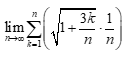
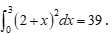
Which of the following integral expressions is equal to

There were 4 answer choices that we will consider in a minute.

To the best of my recollection the last time a question of this type appeared on the AP Calculus exams was in 1997, when only about 7% of the students taking the exam got it correct. Considering that by random guessing about 20% should have gotten it correct, this was a difficult question. This question, the “radical 50” question is at the end of this post.

The first key to answering the question is to recognize the limit as a Riemann sum. In general, a right-side Riemann sum for the function f on the interval [a, b] with n equal subdivisions has the form:

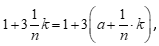
To evaluate the limit and express it as an integral, we must identify, a, b, and f. I usually begin by looking for (b – a)/n. In this problem (b – a)/n = 1/n and from this conclude that b – a = 1, so b = a + 1.

Then rewriting the radicand as

It appears that the function is

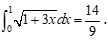
and the limit is

.This is the first answer choice. The choices are:

In this example, choices B, C, and D can be eliminated as soon as we determine that b = a + 1, but that is not always the case.

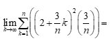
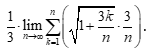
Let’s consider another example:

Example 2:

As before consider (b – a)/n = 3/n implies that b = a + 3. And the function appears to be

on the interval [0, 3], so the limit is

BUT

What is we take a = 2. If so, the limit is

And now one of the “problems” with this kind of question appears: the answer written as a definite integral is not unique!

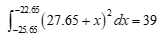
Not only are there two answers, but there are many more possible answers. These two answers are horizontal translations of each other, and many other translations are possible, such as

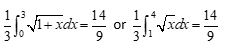
Returning to example 1, using something like a u-substitution, we can rewrite the original limit as .

Now b = a + 3 and the limit could be either

You will probably have your students write Riemann sums with a small value of n when you are teaching Riemann sums leading up to the Fundamental Theorem of Calculus. You can make up problems like this these by stopping after you get to the limit, giving your students just the limit, and have them work backwards to identify the function(s) and interval(s). You could also give them an integral and ask for the associated Riemann sum. Question writes call a question like this a reversal question, since the work is done in reverse of the usual way.

Another example appears in the 2016 “Practice Exam” available at your audit website. It is question AB 30. That question gives the definite integral and asks for the associate Riemann sum; a slightly different kind of reversal. Since this type of question appears in both the CED examples and the practice exam, chances of it appearing on future exams look good.

Critique of the problem

I’m not sure if this type of problem has any practical or real-world use. Certainly, setting up a Riemann sum is important and necessary to solve a variety of problems. After all, behind every definite integral there is a Riemann sum. But starting with a Riemann sum and finding the function and interval does not seem to me to be of practical use.

The CED references this question to MPAC 1: Reasoning with definitions and theorems, and to MPAC 5: Building notational fluency. They are appropriate, but still is the question ever done outside a test or classroom setting?

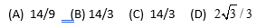
Another, bigger, problem is that the answer choices to Example 1 force the student to do the problem in a way that gets one of the answers. It is perfectly reasonable for the student to approach the problem a different way, and get another correct answer that is not among the choices. This is not good. The question could be fixed by giving the answer choices as numbers. These are the numerical values of the 4 choices:

As you can see that presents another problem.

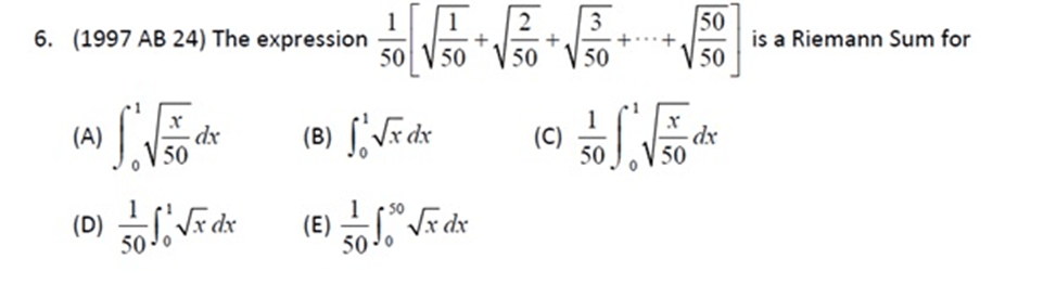
Finally, here is the question from 1997, for you to try:

Answer B. Hint n = 50

_______________________________

Note: The original of this post was lost somehow. I’ve recreated it here. Sorry if anyone was inconvenienced. LMc May 5, 2024

Riemann Sum & Table Problems (Type 5)

Posted on March 25, 2022 by Lin McMullin

AP Questions Type 5: Riemann Sum & Table Problems

Information given in tables may be used to test a variety of ideas in calculus including analysis of functions, accumulation, theory and theorems, and position-velocity-acceleration, among others. Numbers and working with numbers are part of the Rule of Four and table problems are one way they are tested. This question often includes an equation in a latter part of the problem that refers to the same situation.

What students should be able to do:

Find the average rate of change over an interval
Approximate the derivative using a difference quotient. Use the two values closest to the number at which you are approximating. This amounts to finding the slope or rate of change. Show the quotient even if you can do the arithmetic in your head and even if the denominator is 1.
Use a left-, right-, or midpoint- Riemann sums or a trapezoidal approximation to approximate the value of a definite integral using values in the table (typically with uneven subintervals). The Trapezoidal Rule, per se, is not required; it is expected that students will add the areas of a small number of trapezoids without reference to a formula.
Average value, average rate of change, Rolle’s theorem, the Mean Value Theorem, and the Intermediate Value Theorem. (See 2007 AB 3 – four simple parts that could be multiple-choice questions; the mean on this question was 0.96 out of a possible nine points.)
These questions are usually presented in context and answers should be in that context. The context may be something growing (changing over time) or linear motion.
Use the table to find a value based on the Mean Value Theorem (2018 AB 4(b)) or Intermediate Value Theorem. Also, 2018 AB 4 (d) asked a related question based on a function given by an equation.
Unit analysis.

Dos and Don’ts

Do: Remember that you do not know what happens between the values in the table unless additional information is given. For example, do not assume that the largest number in the table is the maximum value of the function, or that the function is decreasing between two values just because a value is less than the preceding value.

Do: Show what you are doing even if you can do it in your head. If you’re finding a slope, show the quotient even if the denominator is 1.

Do Not do arithmetic: A long expression consisting entirely of numbers such as you get when doing a Riemann sum, does not need to be simplified in any way. If you simplify a correct answer incorrectly, you will lose credit.

Do Not leave expression such as R(3) – pull its numerical value from the table.

Do Not: Find a regression equation and then use that to answer parts of the question. While regression is perfectly good mathematics, regression equations are not one of the four things students may do with their calculator. Regression gives only an approximation of our function. The exam is testing whether students can work with numbers.

This question typically covers topics from Unit 6 of the CED but may include topics from Units 2, 3, and 4 as well.

Free-response examples:

2007 AB 3 (4 simple parts on various theorems, yet the mean score was 0.96 out of 9),
2017 AB 1/BC 1, and AB 6,
2016 AB 1/BC 1
2018 AB 4
2021 AB 1/ BC 1
2022 AB4/BC4 – average rate of change, IVT, Rieman sum, Related Rate (part (d) good question)
2023 AB 1/ BC 1 – Right Riemann sum, slope equals zero (may be done by max/min analysis, MVT, or Rolle’s Theorem), Equation extension – average value, meaning of derivative.

Multiple-choice questions from non-secure exams:

2012 AB 8, 86, 91
2012 BC 8, 81, 86 (81 and 86 are the same on both the AB and BC exams)

Revised March 12, 2021, March 25, 2022, June 6, 2023

A Calculus Journey

Posted on November 9, 2021 by Lin McMullin

I think that the path leading up to and including the Fundamental Theorem of Calculus (FTC) is one of the most beautiful walks in mathematics. I have written several posts about it. You will soon be ready to travel that path with your students. (I always try to post on topics shortly before most teachers will get to them, so that you have some time to consider them and work the ideas you like into your lessons.)

Here is an annotated list of some of the posts to guide you on your journey.

Working Towards Riemann Sums gives the preliminary definitions you will need to define and discuss Riemann sums.

Riemann Sums defines the several Riemann sums often used in the calculus left-side sums, right-side sums, midpoint sums and the trapezoidal sums. “The Area Under a Curve” in the iPad app A Little Calculus is a great visual display of these and shows what happens as you use more subintervals.

The Definition of the Definite Integral gives the definition of the definite integral as the limit of any Riemann sum. As with any definition, there is nothing to prove or argue about here. The thing to remember is that the limit of the Riemann sum and the definite integral are the same thing. Behind any definite integral is a Riemann sum. The advantage of the definition’s integral notation is that it shows the interval involved which the Riemann sum does not. (Any Riemann sum may be represented by many definite integrals. See Good Question 11 – Riemann Reversed.)

Foreshadowing the FTC is an example of how a definite integral may be evaluated. It is long and has a lot of notation, so you may not want to use this.

The Fundamental Theorem of Calculus is where the path leads. This post develops the FTC based on the other “big” idea of the calculus: the Mean Value Theorem. (I think the form here is preferable to the usual book notation that uses F(x) and its derivate f (x).)

Y the FTC? Tries to answer the question of what’s so important about the FTC. Example 1: The verbal interpretation of the FTC (the integral of a rate of change is the net amount of change over the interval.) will soon be used in many practical applications. While example 2 shows how the FTC allows one to evaluate a definite integral and, therefore the Riemann sum it represents, by evaluating a function whose derivative is the integrand (its antiderivative).

More About the FTC presents examples leading up to the other form of the FTC: the derivative of the integral is the integrand).

At this point you may go in the direction of learning how to find antiderivatives or working on applications. (See Integration itinerary.)

Bon Voyage!

The Old Pump

Posted on November 5, 2021 by Lin McMullin

A tank is being filled with water using a pump that is old and slows down as it runs. The table below gives the rate at which the pump pumps at ten-minute intervals. If the tank initially has 570 gallons of water in it, approximately how much water is in the tank after 90 minutes?

Elapsed time (minutes)	0	10	20	30	40	50	60	70	80	90
Rate (gallons / minute)	42	40	38	35	35	32	28	20	19	10

And so, integration begins.

Ask your students to do this problem alone. When they are ready (after a few minutes) collect their opinions. They will not all be the same (we hope, because there is more than one reasonable way to approximate the amount). Ask exactly how they got their answers and what assumptions they made. Be sure they always include units (gallons). Here are some points to make in your discussion – points that we hope the kids will make and you can just “underline.”

1. Answers between 3140 and 3460 gallons are reasonable. Other answers in that range are acceptable. They will not use terms like “left-sum”, “right sum” and “trapezoidal rule” because they do not know them yet, but their explanations should amount to the same thing. An answer of 3300 gallons may be popular; it is the average of the other two, but students may not have gotten it by averaging 3140 and 3460.
2. Ask if they think their estimate is too large or too small and why they think that.
3. Ask what they need to know to give a better approximation – more and shorter time intervals.
4. Assumptions: If they added 570 + 42(10) + 40(10) + … +19(10) they are assuming that the pump ran at each rate for the full ten minutes and then suddenly dropped to the next. Others will assume the rate dropped immediately and ran at the slower rate for the 10 minutes. Some students will assume the rate dropped evenly over each 10-minute interval and use the average of the rates at the ends of each interval (570 + 41(10) + 39(10) + … 14.5(10) = 3300).
5. What is the 570 gallons in the problem for? Well, of course to foreshadow the idea of an initial condition. Hopefully, someone will forget to include it and you can point it out.
6. With luck someone will begin by graphing the data. If no one does, you should suggest it; (as always) to help them see what they are doing graphically. They are figuring the “areas” of rectangles whose height is the rate in gallons/minute and whose width is the time in minutes. Thus the “area” is not really an area but a volume (gal/min)(min) = gallons). In addition to unit analysis, graphing is important since you will soon be finding the area between the graph of a function and the x-axis in just this same manner.

Follow up: Flying to Integrationland

Be sure to check the “Thoughts on ‘The Old Pump'” in the comments section below.

Revised from a post of November 30, 2012.

Unit 6 – Integration and Accumulation of Change

Posted on November 2, 2021 by Lin McMullin

Unit 6 develops the ideas behind integration, the Fundamental Theorem of Calculus, and Accumulation. (CED – 2019 p. 109 – 128). These topics account for about 17 – 20% of questions on the AB exam and 17 – 20% of the BC questions.

Topics 6.1 – 6.4 Working up to the FTC

Topic 6.1 Exploring Accumulations of Change Accumulation is introduced through finding the area between the graph of a function and the x-axis. Positive and negative rates of change, unit analysis.

Topic 6.2 Approximating Areas with Riemann Sums Left-, right-, midpoint Riemann sums, and Trapezoidal sums, with uniform partitions are developed. Approximating with numerical methods, including use of technology are considered. Determining if the approximation is an over- or under-approximation.

Topic 6.3 Riemann Sums, Summation Notation and the Definite Integral. The definition integral is defined as the limit of a Riemann sum.

Topic 6.4 The Fundamental Theorem of Calculus (FTC) and Accumulation Functions Functions defined by definite integrals and the FTC.

Topic 6.5 Interpreting the Behavior of Accumulation Functions Involving Area Graphical, numerical, analytical, and verbal representations.

Topic 6.6 Applying Properties of Definite Integrals Using the properties to ease evaluation, evaluating by geometry and dealing with discontinuities.

Topic 6.7 The Fundamental Theorem of Calculus and Definite Integrals Antiderivatives. (Note: I suggest writing the FTC in this form $displaystyle int_{a}^{b}{{{f}'left( x right)}}dx=fleft( b right)-fleft( a right)$ because it seem more efficient then using upper case and lower case f.)

Topics 6.5 – 6.14 Techniques of Integration

Topic 6.8 Finding Antiderivatives and Indefinite Integrals: Basic Rules and Notation. Using basic differentiation formulas to find antiderivatives. Some functions do not have closed-form antiderivatives. (Note: While textbooks often consider antidifferentiation before any work with integration, this seems like the place to introduce them. After learning the FTC students have a reason to find antiderivatives. See Integration Itinerary

Topic 6.9 Integration Using Substitution The u-substitution method. Changing the limits of integration when substituting.

Topic 6.10 Integrating Functions Using Long Division and Completing the Square

Topic 6.11 Integrating Using Integration by Parts (BC ONLY)

Topic 6.12 Integrating Using Linear Partial Fractions (BC ONLY)

Topic 6.13 Evaluating Improper Integrals (BC ONLY) Showing the work requires students to show correct limit notation.

Topic 6.14 Selecting Techniques for Antidifferentiation This means practice, practice, practice.