Lin McMullin’s Theorem

Posted on July 10, 2013 by Lin McMullin

Mathematics more often tends to delight when it exhibits an unanticipated result rather than conforming to … expectations. In addition, the pleasure derived from mathematics is related in many cases to the surprise felt upon the perception of totally unexpected relationships and unities.

– Mario Livio, The Golden Ratio

I have a theorem named after me. I did not name it, but I did prove it – well more like I tripped over it. It is a calculus related idea. Here is how it came about. I say “came about” because as you will see I did not set out to prove it. I just sort of fell in my lap as I was working on something else.

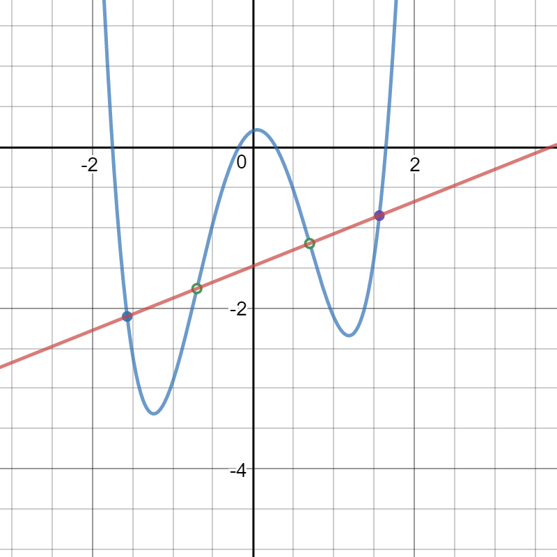
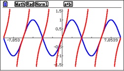
I was trying to do an animation of an idea that I had heard about: If you have a fourth degree, or quartic, polynomial with a “W” shape it has two points of inflection. If you draw a line through the points of inflection three regions enclosed by the line and the polynomial’s graph are formed. The areas of these regions are in the ratio of 1:2:1. In order to make the animation work I needed the general coordinates of the four points where the line intersects the quartic.

The straightforward way to proceed would be to write a general fourth degree polynomial,

$f\left( x \right)={{c}_{4}}{{x}^{4}}+{{c}_{3}}{{x}^{3}}+{{c}_{2}}{{x}^{2}}+{{c}_{1}}x+{{c}_{0}}$

differentiate it twice to find the second derivative. Then find the zeros of the second derivative (by the quadratic formula), write the equation of the line through them, and then find where else the line intersects the quartic. Without even starting I realized that even with a CAS the algebra and equation solving was going to be really fun (Not!). So, I decided on an alternative approach.

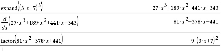
I decided to let the zeros of the second derivative be x = a and x = b, then at least they would be easy to work with. Then the second derivative is $\displaystyle {{f}'}'\left( x \right)=12{{c}_{4}}\left( x-a \right)\left( x-b \right)$ where the ${{c}_{4}}$ is the leading coefficient of the quartic and the 12 comes from differentiating twice.

I integrated to get the first derivative and added ${{c}_{1}}$ , the coefficient of the linear term, as the constant of integration. I integrated again and added ${{c}_{0}}$ , the constant term. as the constant of integration. This resulted in the original quartic function:

$\displaystyle f\left( x \right)={{c}_{4}}{{x}^{4}}-2\left( a+b \right){{c}_{4}}{{x}^{3}}+6ab{{c}_{4}}{{x}^{2}}+{{c}_{1}}x+{{c}_{0}}$

Then I wrote the equation of y(x) the line through the points of inflection. It is too long to copy, but you may see it in the screen capture at the end of the post. (That is what is nice about a CAS: you really do not have to worry about how complicated things are.)

Then I solved the equation $f\left( x \right)=y\left( x \right)$ . Two of the solutions are x = a and x = b as I expected. (This means that you could do synthetic division by hand since you know two of the roots.) The other two I did not expect. They are:

$\displaystyle {{x}_{1}}=\frac{1+\sqrt{5}}{2}a+\frac{1-\sqrt{5}}{2}b$ and $\displaystyle {{x}_{2}}=\frac{1+\sqrt{5}}{2}b+\frac{1-\sqrt{5}}{2}a$

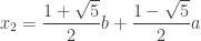
And that’s when I stopped astonished! Those numbers are the Golden Ratio $\Phi =\frac{1+\sqrt{5}}{2}$ , and its reciprocal $\phi ={{\Phi }^{-1}}=\frac{1-\sqrt{5}}{2}$ . So the roots are $\Phi a+\phi b$ and $\Phi b+\phi a$ . How did they get there?

To this day I have no idea why the Golden Ratio should be so involved with quartic polynomials, but there they are in every quartic!

There were no assumptions made about a and b – they could be Complex numbers. In that case there are no points of inflection, but the “line” and the quartic still will have the same value at the four points.

October 16, 2022 Update: If the solutions of $\displaystyle {y}''=0$ are the Complex conjugates $\displaystyle a=\alpha +\beta i$ and $\displaystyle b=\alpha -\beta i$ then $\displaystyle {{x}_{1}}=\alpha +\sqrt{5}\beta i$ and $\displaystyle {{x}_{2}}=\alpha -\sqrt{5}\beta i$ . When graphed on an Argand diagram the four points are collinear on the vertical line at $\displaystyle x=\alpha$

This was all in 2013 and until just this year I never checked the ratio of the areas. (They check.)

Here is a CAS printout of the entire computation.

An interactive Desmos demo of this can be found here

October 16, 2022, Update: If the solutions of $\displaystyle {y}''=0$ are the Complex conjugates $\displaystyle a=\alpha +\beta i$ and $\displaystyle b=\alpha -\beta i$ then $\displaystyle {{x}_{1}}=\alpha +\sqrt{5}\beta i$ and $\displaystyle {{x}_{2}}=\alpha -\sqrt{5}\beta i$ . When graphed on an Argand diagram the four points are collinear on the vertical line at $\displaystyle x=\alpha$

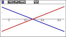
November 10, 2020, Update: I received an email this week form Dominique Laurain, a computer science and applied math engineer from France, who describes himself as a mathematics hobbyist. He discovered another interesting relationship between the coordinates of the x-coordinates of the four points on the line described above. The four points on the line through the points of inflection of a fourth degree polynomial with Real roots in the drawing above from left to right are p, q, r, and s. The coordinates of the points of inflection are a and b as in the post above.

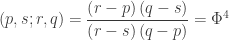
One, of several, cross-ratios of four points with x-coordinates of p, q r, and s is defined as

$\displaystyle (p,s;r,q)=\frac{{\left( {r-p} \right)\left( {q-s} \right)}}{{\left( {r-s} \right)\left( {q-p} \right)}}$ .

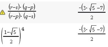
Dominique Laurin discovered that $\displaystyle (p,s;r,q)=\frac{{\left( {r-p} \right)\left( {q-s} \right)}}{{\left( {r-s} \right)\left( {q-p} \right)}}={{\Phi }^{4}}$

The computation is shown in the figure below.

There are 24 other cross-ratios depending on the order of the points. In groups of 4, the 24 possible orders are equal to 6 related values. See the cross-ratio link above above. For example, the cross-ratio in the order (s, p; r, q) is ${{\varphi }^{4}}$

Also, $(q,r;s,p)={{\Phi }^{4}}$

Other interesting information:

The Golden Ratio also appears in cubic equations. See the Tashappat – McMullin theorem here.

“Quartic Polynomials and the Golden Ratio” by Harald Totland of the Royal Norwegian Naval Academy. (June 2009)

Speaking of the Golden Ratio, the Calculus Humor website has a nice feature on the Golden Ratio in logos. To view it click here.

Link for cross-ratios

Revised and updated July 20 and 23, 2017, November 10, 2020

Experimenting with CAS – Chain Rule

Posted on July 3, 2013 by Lin McMullin

Discovering things in mathematics can be facilitated by using a computer algebra system (CAS) available on many handheld calculators and computer apps. A CAS can provide good data with which to draw conclusions. You can do “experiments” by producing the results with a CAS and looking for patterns. As an example, let’s look at how you and your students might discover the chain rule for derivatives.

One of the ways you could introduce the chain rule is to ask your class to differentiate something like (3x + 7)². Not knowing about the chain rule, just about the only way to proceed is to expand the expression to 9x² + 42x + 49 and differentiate that: 18x + 42 and then factor 6(3x + 7). Then you show how this relates to the power rule and where the “extra” factor of 3 comes from differentiating the (3x + 7). You really cannot a much more complicated example, say a third or fourth power, because the algebra gets complicated very fast.

Or does it?

Suggest your students use a CAS to do the example above this time using the third power. The output might look like this:

But even better: what we want is just the answer. Who cares about all the algebra in between? Try a few powers until the pattern become obvious.

Now we have some good data to work with. Can you guess the pattern?

Nor sure where the “extra” factor of 3 comes from? Try changing the 3 in the original and keep the exponent the same.

Now can you guess the chain rule? See if what you thought is right by changing only the inside exponent.

Then you can try some others:

CAS D

You can count on the CAS giving you the correct data (answers). Do enough experiments until the chain rule pattern becomes clear.

But I think the big thing is not the chain rule, but that the students are learning how to experiment in mathematics situations. In these we started by changing only the outside power. Then we kept the power the same power and changed the coefficient of the linear factor. Then we changed the power inside power, each time seeing if our tentative rule for differentiating composite function was correct and adjusting it if it was not. Finally we tried a variety of different expressions. You change things. Not big things but little things. You don’t jump from one trial to something very different, only something a little different.

You can do the same thing for the product rule, the quotient rule, maybe some integration rules and so on. You have accomplished your goal when the students can produce the data they need without your suggestions.

But be aware: sometimes this can lead to unexpected results. Does the pattern hold here?

Or here?

Hint: $\frac{7}{3.2}=2.1875$ and $3{{\left( 3.2 \right)}^{3}}=98.304$

Revised 8-25-17

Locally Linear L’Hôpital

Posted on May 31, 2013 by Lin McMullin

I’ll begin with a lemma. (I like to do a lemma now and then if for no other reason than having an excuse to explain what a lemma is – a simple theorem that is used in proving the main theorem.)

Lemma: If two lines intersect on the x-axis, then for any x the ratio of their y-coordinates is equal to the ratio of their slopes.

Proof: Two lines with slopes of m₁ and m₂ that intersect at (a, 0) on the x-axis have equations y₁ = m₁(x – a) and y₂ = m₂(x – a). Then

$\displaystyle \frac{{{y}_{1}}}{{{y}_{2}}}=\frac{{{m}_{1}}\left( x-a \right)}{{{m}_{2}}\left( x-a \right)}=\frac{{{m}_{1}}}{{{m}_{2}}}$

L’Hôpital’s Rule (Theorem): If f and g are differentiable near x = a and f(a) = g(a) = 0, then

$\displaystyle \underset{x\to a}{\mathop{\lim }}\,\frac{f\left( x \right)}{g\left( x \right)}=\underset{x\to a}{\mathop{\lim }}\,\frac{{f}'\left( x \right)}{{g}'\left( x \right)}$

if the limit exists.

The fact that f(a) = g(a) = 0 means that the two functions intersect on the x-axis at (a, 0). For example, the functions f(x) = tan(x) and g(x) = sin(x) have this property at $\left( \pi ,0 \right)$ .

Figure 1. y = tan(x) in red and y = sin(x) in blue

Now zoom-in several times centered at $\left( \pi ,0 \right)$ .

Figure 2. The previous graph zoomed in.

Whoa!

That looks like lines!!

It’s the local linearity property of differentiable functions – if you zoom-in enough any differentiable function eventually looks linear. So maybe near $\left( \pi ,0 \right)$ the lemma applies. The only difference is that the slopes of the “lines” are the derivatives so

$\displaystyle \underset{x\to a}{\mathop{\lim }}\,\frac{f\left( x \right)}{g\left( x \right)}=\underset{x\to a}{\mathop{\lim }}\,\frac{{f}'\left( x \right)}{{g}'\left( x \right)}$

Now that does not quite prove L’Hôpital’s Rule, but it should give you and your students a good idea of why L’Hôpital’s Rule is true.

Then in our example:

$\displaystyle \underset{x\to \pi }{\mathop{\lim }}\,\frac{\tan \left( x \right)}{\sin \left( x \right)}=\underset{x\to \pi }{\mathop{\lim }}\,\frac{\frac{1}{{{\left( \cos \left( x \right) \right)}^{2}}}}{\cos \left( x \right)}=\underset{x\to \pi }{\mathop{\lim }}\,\frac{1}{{{\left( \cos \left( x \right) \right)}^{3}}}=\frac{1}{{{\left( \cos \left( \pi \right) \right)}^{3}}}=-1$

But isn’t that obvious from Figure 2?

Think about it.

Logarithms

Posted on February 6, 2013 by Lin McMullin

Students first encounter logarithms in Algebra 2 or their last pre-calculus course. They are usually defined as exponents and their properties “proven” by reference to the corresponding properties of exponents. This is good enough at the time, but in calculus we are ready to define logarithms properly. The result is the definition in terms of a function defined by an integral.

In fact, the definition flows naturally from the properties of inverse functions (no pun intended, because the flow is quite natural). But is this a definition? Or a proof? The solution of certain differential equations discussed in my last post may be used to derive the logarithm function.

Let’s begin by pretending we know nothing about logarithms, and investigate the inverse of e^x. (See The Derivative of Exponential Functions)

This function e^x contains points of the form $\left( X,{{e}^{X}} \right)$ so its inverse will contain points of the form $\left( {{e}^{X}},X \right)$ , which, since we like the first coordinate of functions to be x, we may also call $\left( x,\ln \left( x \right) \right)$ , where ln(x) will be the name of the inverse of e^x. Remember, at the moment ln(x) is just a notation for the inverse of e^x, we do not know anything about logarithms (yet).

So $\left( {{e}^{X}},X \right)$ = $\left( x,\ln \left( x \right) \right)$ and $X\ne x$ . For example, (0, 1) is a point on e^X, so (1, 0) is a point on the ln(x) function, and so ln(1) = 0.

In a previous post we defined the number e and the function e^x in such a way that $\displaystyle \frac{d}{dx}{{e}^{x}}={{e}^{x}}$ . Now, at $\left( X,{{e}^{X}} \right)$ the derivative is e^X, so at the corresponding point on its inverse, $\left( {{e}^{X}},X \right)$ , the derivative is the reciprocal of the derivative of e^X which is $\frac{1}{{{e}^{X}}}=\frac{1}{x}$ . That is

$\displaystyle \frac{d}{dx}\ln \left( x \right)=\frac{1}{x}$

We can use this idea to define ln(x) as a function defined by an integral. Solving the differential equation by the method suggested in a recent post we get:

$\displaystyle \ln \left( x \right)=\ln \left( a \right)+\int_{a}^{x}{\frac{1}{t}dx}$

We can pick any positive number for a and a convenient one is the one we already found a = 1 where ln(1) = 0, so

$\displaystyle \ln \left( x \right)=\int_{1}^{x}{\frac{1}{t}dx},\quad x>0$

This then is the “official definition” of the natural logarithm function. The domain is x > 0 (the range of e^x) and the range is all real numbers (the domain of e^x).

Graphically, ln(x) is the area between the graph of $\displaystyle \frac{1}{t}$ and the t-axis between 1 and x. If $0<x<1$ , then $\ln \left( x \right)<0$ and if $x>1$ , $\ln \left( x \right)>0$ .

From this definition we can prove all the familiar properties of logarithms $\left( \ln \left( ab \right)=\ln \left( a \right)+\ln \left( b \right)\text{ etc}\text{.} \right)$ and show that this is a function of the kind we called “logarithm” all along. This is in all the textbooks so I will not go into this here.

One of these properties tells us that for $a>0\text{ and }a\ne 1$ , $\displaystyle {{\log }_{a}}\left( x \right)=\frac{\ln \left( x \right)}{\ln \left( a \right)}$ and since ln(a) is a constant

$\displaystyle {{\log }_{a}}\left( x \right)=\frac{1}{\ln \left( a \right)}\int_{1}^{x}{\frac{1}{t}dt}$

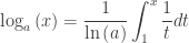
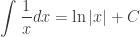
Finally, you will see this antiderivative formula: $\displaystyle \int_{{}}^{{}}{\frac{1}{x}dx=\ln \left| x \right|+C}$ . The absolute value sign is to remind you that the argument of the logarithm function must be positive, since in some situations x itself may be negative.

Revised slightly 8-28-2018

The Derivatives of Exponential Functions

Posted on November 21, 2012 by Lin McMullin

Our problem for today is to differentiate a^x with the (usual) restrictions that a is a positive number and not equal to 1. The reasoning here is very different from that for finding other derivatives and therefore I hope you and your students find it interesting.

The definition of derivative followed by a little algebra gives tells us that

$\displaystyle \frac{d}{dx}{{a}^{x}}=\underset{h\to 0}{\mathop{\lim }}\,\frac{{{a}^{x+h}}-{{a}^{x}}}{h}=\underset{h\to 0}{\mathop{\lim }}\,\frac{{{a}^{x}}{{a}^{h}}-{{a}^{x}}}{h}={{a}^{x}}\underset{h\to 0}{\mathop{\lim }}\,\frac{{{a}^{h}}-1}{h}$ .

Since the limit in the expression above is a number, we observe that the derivative of a^x is proportional to a^x. And also, each value of a gives a different constant. For example if a = 5 then the limit is approximately 1.609438, and so $\displaystyle \frac{d}{{dx}}{{5}^{x}}\approx \left( {1.609438} \right){{5}^{x}}$ .

I determined this by producing a table of values for the expression in the limit near x = 0. You can do the same using a good calculator, computer, or a spreadsheet.

h $\frac{{{5}^{h}}-1}{h}$

-0.00000030 1.60943752

-0.00000020 1.60943765

-0.00000010 1.60943778

0.00000000 undefined

0.00000010 1.60943804

0.00000020 1.60943817

0.00000030 1.60943830

That’s kind of messy and would require us to find this limit for whatever value of a we were using. It turns out that by finding the value of a for which the limit is 1 we can fix this problem. Your students can do this for themselves by changing the value of a in their table until they get the number that gives a limit of 1.

Okay, that’s going to take a while, but may be challenging. The answer turns out to be close to 2.718281828459045…. Below is the table for this number.

h $\frac{{{a}^{h}}-1}{h}$

-0.00000030 0.99999985

-0.00000020 0.99999990

-0.00000010 0.99999995

0.00000000 undefined

0.00000010 1.00000005

0.00000020 1.00000010

0.00000030 1.00000015

Okay, I cheated. The number is, of course, e. Thus,

$\displaystyle \frac{d}{{dx}}{{e}^{x}}={{e}^{x}}\left( {\underset{{h\to 0}}{\mathop{{\lim }}}\,\frac{{{{e}^{h}}-1}}{h}} \right)={{e}^{x}}(1)={{e}^{x}}$ .

The function e^x is its own derivative!

And from this we can find the derivatives of all the other exponential functions. First, we define a new function (well maybe not so new) which is the inverse of the function e^x called ln(x), the natural logarithm of x. (For more on this see Logarithms.) Then a = e^ln(a) and a^x = (e^ln(a))^x = e^(ln(a)x). Then using the Chain Rule, the derivative is

$\frac{d}{dx}{{a}^{x}}={{e}^{(\ln (a))x}}\ln (a)={{\left( {{e}^{\ln (a)}} \right)}^{x}}\ln (a)$

$\frac{d}{dx}{{a}^{x}}={{a}^{x}}\ln \left( a \right)$

Finally, going back to the first table above where a = 5, we find that the limit we found there 1.609438 = ln(5).

For a video on this topic click here.

Revised 8-28-2018, 6-2-2019

Motion Problems: Same Thing, Different Context

Posted on November 16, 2012 by Lin McMullin

Calculus is about things that are changing. Certainly, things that move are changing, changing their position, velocity and acceleration. Most calculus textbooks deal with things being dropped or thrown up into the air. This is called uniformly accelerated motion since the acceleration is due to gravity and is constant. While this is a good place to start, the problems are by their nature, somewhat limited. Students often know all about uniformly accelerated motion from their physics class.

The Advanced Placement exams take motion problems to a new level. AB students often encounter particles moving along the x-axis or the y-axis (i.e. on a number line) according to some function that gives the particle’s position, velocity or acceleration. BC students often encounter particles moving around the plane with their coordinates given by parametric equations or its velocity given by a vector. Other times the information is given as a graph or even in a table of the position or velocity. The “particle” may become a car, or a rocket or even chief readers riding bicycles.

While these situations may not be all that “real”, they provide excellent ways to ask both differentiation and integration questions. but be aware that they are not covered that much in some textbooks; supplementing the text may be necessary.

The main derivative ideas are that velocity is the first derivative of the position function, acceleration is the second derivative of the position function and the first derivative of the velocity. Speed is the absolute value of velocity. (There will be more about speed in the next post.) The same techniques used to find the features of a graph can be applied to motion problems to determine things about the moving particle.

So the ideas are not new, but the vocabulary is. The table below gives the terms used with graph analysis and the corresponding terms used in motion problem.

Vocabulary: Working with motion equations (position, velocity, acceleration) you really do all the same things as with regular functions and their derivatives. Help students see that while the vocabulary is different, the concepts are the same.

Function Linear Motion

Value of a function at x position at time t

First derivative velocity

Second derivative acceleration

Increasing moving to the right or up

Decreasing moving to the left or down

Absolute Maximum farthest right

Absolute Minimum farthest left

yʹ = 0 “at rest”

yʹ changes sign object changes direction

Increasing & cc up speed is increasing

Increasing & cc down speed is decreasing

Decreasing & cc up speed is decreasing

Decreasing & cc down speed is increasing

Speed absolute value of velocity

Inverses Graphically and Numerically

Posted on November 14, 2012 by Lin McMullin

In this final post in this series on inverses we consider the graphical and numerical concepts related to the derivative of the inverse and look at an important formula.

To make the notation a little less messy, let’s let g(x) = f ^-1(x). Then we know that f (g(x))= x. Differentiating this implicitly gives

${f}'\left( g\left( x \right) \right){g}'\left( x \right)=1$
$\displaystyle {g}'\left( x \right)=\frac{1}{{f}'\left( g\left( x \right) \right)}$

Great formula, but one I’ve never been able to memorize and use correctly! It’s my least favorite formula, because I’m never quite sure what to substitute for what.

The graph shows a function and its inverse. It really doesn’t matter which is which, since inverse functions come in pairs: the inverse of the inverse is the original function.

Notice that the graphs are symmetric to y = x. At two points, one of which is the image of the other after reflecting over the line y = x, a tangent segment has been drawn. This segment is the hypotenuse of the “slope triangle” which is also drawn. The ratio of the vertical side of this triangle to the horizontal side is the slope (i.e. the derivative) of the tangent line.

The two triangles are congruent, so that the horizontal side of one triangle is congruent to the vertical side of the other, and vice versa. Thus the slope (the derivative) of the one tangent segment is the reciprocal of the other.

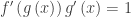
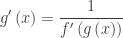
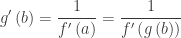
If (a, b) is a point on a function and the derivative at this point is ${f}'\left( a \right)$ , then the point (b, a) is on the function’s inverse and the derivative here is $\displaystyle \frac{1}{{f}'\left( a \right)}$ . This is just what my least favorite formula says: if f ^-1 (x) = g(x), then a = g(b) and $\displaystyle {g}'\left( b \right)=\frac{1}{{f}'\left( a \right)}=\frac{1}{{f}'\left( g\left( b \right) \right)}$ .

What you really need to know is:

At corresponding points on a function and its inverse, the derivatives are reciprocals of each other.

This is what my least favorite formula says.

The AP exams have a clever way of testing this. (The stem may give a few more values to throw you off, or the values may be in a table.)

Given that $f\left( 2 \right)=5\text{ and }{f}'\left( 2 \right)=3$ and g is the inverse of f, Find ${g}'\left( 5 \right)$ .

The solution is reasoned this way: (5, ?) is a point on g. The corresponding point on f is (?, 5) = (2, 5). The derivative of f at this point is 3, therefore the derivative at (5, 2) on g is ${g}'\left( 5 \right)=\tfrac{1}{3}$ .

Easy!

Teaching Calculus

The pleasure lies not in discovering the truth, but in searching for it.

Category Archives: Derivative Theory

Lin McMullin’s Theorem

Experimenting with CAS – Chain Rule

Locally Linear L’Hôpital

Logarithms

The Derivatives of Exponential Functions

Motion Problems: Same Thing, Different Context

Inverses Graphically and Numerically

Share this:

Share this:

Share this:

Share this:

Share this:

Share this:

Share this: