Every Spring I have a lot of fun proofreading Audrey Weeks’ new Calculus in Motion illustrations for the most recent AP Calculus Exam questions. These illustrations run on Geometers’ Sketchpad. In addition to the exam questions Calculus in Motion (and its companion Algebra in Motion) include separate animations illustrating most of the concepts in calculus and algebra. This is a great resource for your classes.
The proofreading and the cross-country conversations with Audrey give me a chance to learn more about the questions.
This year, I really got into 2018 AB 6, the differential equation question. I wrote an exploration (or as the kids would say “worksheet”) on a function very similar to the differential equation in that question. The exploration, which is rather long, includes these topics:
- Finding the general solution of the differential equation by separating the variables
- Checking the solution by substitution
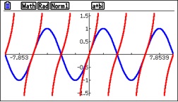
- Using a graphing utility to explore the solutions for all values of the constant of integration, C
- Finding the solutions’ horizontal and vertical asymptotes
- Finding several particular solutions
- Finding the domains of the particular solutions
- Finding the extreme value of all solutions in terms of C
- Finding the second derivative (implicit differentiation)
- Considering concavity
- Investigating a special case or two
I also hope that in working through this exploration students will learn not so much about this particular function, but how to use the tools of algebra, calculus, and technology to fully investigate any function and to find all its foibles.
Students will need to have studied calculus through differential equations before they start the exploration. I will repost it next January for them.
The exploration is here for you to try. Try it before you look at the solutions. It will give you something to do over the summer – well not all summer, only an hour or so.
As always, I appreciate your feedback and comments. Please share them with me using the reply box below.
There will be only occasional, very occasional, posts over the Summer. More regular posting will begin again in August. Enjoy the Explorations, and, more important, enjoy the Summer!

.
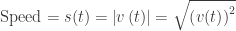 . Then,
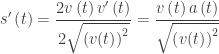
 and speed is increasing when
  and
and  have the same sign, and
  and speed is decreasing when they have different signs.