Introducing Power Series 1

The next few posts will discuss a way to introduce Taylor and Maclaurin series to students. We will kind of sneak up on the idea without mentioning where we are going or using any special terms. In this post we will find a way of approximating a function with a polynomial of any degree we choose. In the next post we will look at the graph of these polynomials and finally suggest some questions for further thought.

Making Better Approximations

Students already know and have been working with the tangent line approximation of a function at a point (a, f(a)):
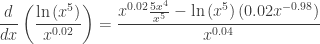
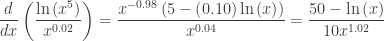
f(x)\approx f\left( a \right)+{f}'\left( a \right)\left( x-a \right)

ln(x):

For the function f\left( x \right)=\ln \left( x \right) at the point (1, 0) ask your students to write the tangent line approximation: y=0+(1)(x-1) .Point out that this line has the same value as  ln(xand its derivative as at (1, 0).

Then suggest that maybe having a polynomial that has the same value, first derivative and second derivative might be a better approximation. Suggest they start with y=a+b\left( x-1 \right)+c{{\left( x-1 \right)}^{2}} and see if they can find values of a, b and c that will make this happen.

Since f\left( 1 \right)=0,{f}'\left( 1 \right)=1\text{ and }{{f}'}'\left( x \right)=-1 we can write

y=a+b\left( x-1 \right)+c{{\left( x-1 \right)}^{2}};\quad y\left( 1 \right)=a+0+0=0;\quad a=0

{y}'=b+2c\left( x-1 \right);\quad {y}'\left( 1 \right)=b+0=\tfrac{1}{1};\quad b=1

{{y}'}'=2c;\quad {{y}'}'\left( 1 \right)=c=-\tfrac{1}{{{1}^{2}}}=-1;\quad c=-\tfrac{1}{2}

y=0+\left( x-1 \right)-\tfrac{1}{2}{{\left( x-1 \right)}^{2}}

Then suggest they try a third degree polynomial starting with y=a+b\left( x-1 \right)+c{{\left( x-1 \right)}^{2}}+d{{\left( x-1 \right)}^{3}}. Proceeding as above, all the numbers come out the same and we find that

\ln \left( x \right)\approx 0+\left( x-1 \right)+\left( -\tfrac{1}{2} \right){{\left( x-1 \right)}^{2}}+\left( \tfrac{1}{3} \right){{\left( x-1 \right)}^{3}}

Then go for a fourth- and fifth-degree polynomial until they discover the patterns. (The signs alternate, and the denominators are the factorial of the exponent.)

See if the class can write a general polynomial of degree N :

 \displaystyle \ln \left( x \right)\approx \sum\limits_{k=1}^{N}{\frac{{{\left( -1 \right)}^{k+1}}}{k}{{\left( x-1 \right)}^{k}}}

sin(x):

Then have the class repeat all this for a new function such as f\left( x \right)=\sin \left( x \right) at the point (0, 0). This could be assigned as homework or group work. Ask them to do enough terms until they see the pattern. There will be patterns similar to ln(x ) and every other term (the even powers) will have a coefficient of zero.

\sin \left( x \right)\approx x-\tfrac{1}{3!}{{x}^{3}}+\tfrac{1}{5!}{{x}^{5}}-\tfrac{1}{7!}{{x}^{7}}+\tfrac{1}{9!}{{x}^{9}}

or in general the polynomial of degree N is

\displaystyle \sin \left( x \right)\approx \sum\limits_{k=1}^{N}{\frac{{{\left( -1 \right)}^{k+1}}}{\left( 2k-1 \right)!}{{x}^{2k-1}}}

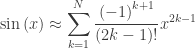
How good is this approximation? Using only the first three terms of the polynomial above you will tell you that. Pretty close: correct to 5 decimal places.  Using four terms gives correct to 7 decimal places when rounded.

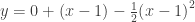
Finally, see if they can generalize this idea to any function f at any point on the function \left( {{x}_{0}},f\left( {{x}_{0}} \right) \right). This time you will not have the various derivatives as numbers, rather they will be expressions like . Work through the powers one at a time to go from y=a+b\left( x-{{x}_{0}} \right)+c{{\left( x-{{x}_{0}} \right)}^{2}}+d{{\left( x-{{x}_{0}} \right)}^{3}}+e{{\left( x-{{x}_{0}} \right)}^{4}}

and so on, until you get to

f\left( x \right)\approx f\left( {{x}_{0}} \right)+\frac{{f}'\left( {{x}_{0}} \right)}{1!}\left( x-{{x}_{0}} \right)+\frac{{{f}'}'\left( {{x}_{0}} \right)}{2!}{{\left( x-{{x}_{0}} \right)}^{2}}

\quad \quad \quad \quad \quad \quad \quad \quad \quad \quad \quad \quad \quad +\cdots +\frac{{{f}^{\left( N \right)}}\left( {{x}_{0}} \right)}{N!}{{\left( x-{{x}_{0}} \right)}^{N}}

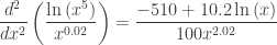
For example the third derivative computation would look like this:

{{{y}'}'}'=3\cdot 2\cdot 1d+4\cdot 3\cdot 2e\left( x-{{x}_{0}} \right)

{{{y}'}'}'\left( {{x}_{0}} \right)=3\cdot 2\cdot 1d+4\cdot 3\cdot 2e(0)={{{f}'}'}'\left( {{x}_{0}} \right)

d=\frac{{{{f}'}'}'\left( {{x}_{0}} \right)}{3!}

The computations here are perhaps a little different than what students have seen, so take your time doing this. Two or even three class days may be necessary.

Notice these things:

  • The first two terms are the tangent line approximation.
  • The various derivatives are numbers that must be calculated.
  • All the terms of any degree are the same as the terms of the previous degree with one additional term.

Next post in this series: Looking at all this graphically.

(Typos in an earlier version of this post have been corrected – LMc)

Inequalities

This is an “extra” post on a technique that students are using a lot right now in graphing functions and working on optimization problems.

In analyzing a derivative to find critical points and then the intervals where the function increases and decreases you need to solve these inequalities. I’ve observed many students solving inequalities the hard way.

By that I mean they will pick a number in each interval between the critical points and then substitute it into the derivative and do a lot of arithmetic to determine whether the derivative is positive or negative. Arithmetic is not necessary, when all you really need is the sign of the derivative. The method I suggest is easier and involves no arithmetic and therefore precludes any arithmetic mistakes

A complete discussion of this idea with examples click here or look on my Resources page.

Speed

Speed is the absolute value of velocity: speed = \left| v\left( t \right) \right| .

This is the definition of speed, but hardly enough to be sure students know about speed and its relationship to velocity and acceleration.

Velocity is a vector quantity; that is, it has both a direction and a magnitude. The magnitude of velocity vector is the speed. Speed is a non-negative number and has no direction associated with it. Velocity has a magnitude and a direction. Speed has the same value and units as velocity; speed is a number. 

The question that seems to trouble students the most is to determine whether the speed is increasing or decreasing. The short answer is

Speed is increasing when the velocity and acceleration have the same sign.

Speed is decreasing when the velocity and acceleration have different signs.

You should demonstrate this in some real context, such as driving a car (see below). Also, you can explain it graphically.

The figure below shows the graph of the velocity v\left( t \right) (blue graph) of a particle moving on the interval 0\le t\le f. The red graph is \left| v\left( t \right) \right|, the speed. The sections where v\left( t \right)<0 are reflected over the x-axis. (The graphs overlap on [b, d].) It is now quite east to see that the speed is increasing on the intervals [0,a], [b, c] and [d,e].

Another way of approaching the concept is this: the speed is the non-directed length of the vertical segment from the velocity’s graph to the t-axis. Picture the segment shown moving across the graph. When it is getting longer (either above or below the t-axis) the speed increases.

Thinking of the speed as the non-directed distance from the velocity to the axis makes answering the two questions below easy:

    1. What are the values of t at which the speed obtains its (local) maximum values? Answer: x = a, c, and e. 
    2. When do the minimum speeds occur?  What are they? Answer: the speed is zero at b and d

Students often benefit from a verbal explanation of all this. Picture a car moving along a road going forwards (in the positive direction) its velocity is positive.

  • If you step on the gas, acceleration pulls you in the direction you are moving and your speed increases. (v > 0, a > 0, speed increases)
  • Going too fast is not good, so you put on your brakes, you now accelerate in the opposite direction (decelerate?), but you are still moving forward, but slower. (v > 0, a < 0, speed decreases)
  • Finally, you stop. Then you shift into reverse and start moving backwards (negative velocity) and you push on the gas to accelerate in the negative direction, so your speed increases. (v < 0, a < 0, speed increases)
  • Then you put on the breaks (accelerate in the positive direction) and your speed decreases again. (v < 0, a > 0, speed decreases)

Here is an activity that will help your students discover this relationship. Give Part 1 to half the class and Part 2 to the other half. Part 3 (on the back of Part 1 and Part 2) is the same for both groups.  – Added 12-19-17

Also see: A Note on Speed for the purely analytic approach.


Update: “A Note on Speed” added 4-21-2018

Motion Problems: Same Thing, Different Context

Calculus is about things that are changing. Certainly, things that move are changing, changing their position, velocity and acceleration. Most calculus textbooks deal with things being dropped or thrown up into the air. This is called uniformly accelerated motion since the acceleration is due to gravity and is constant. While this is a good place to start, the problems are by their nature, somewhat limited. Students often know all about uniformly accelerated motion from their physics class.

The Advanced Placement exams take motion problems to a new level. AB students often encounter particles moving along the x-axis or the y-axis (i.e. on a number line) according to some function that gives the particle’s position, velocity or acceleration.  BC students often encounter particles moving around the plane with their coordinates given by parametric equations or its velocity given by a vector. Other times the information is given as a graph or even in a table of the position or velocity. The “particle” may become a car, or a rocket or even chief readers riding bicycles.

While these situations may not be all that “real”, they provide excellent ways to ask both differentiation and integration questions. but be aware that they are not covered that much in some textbooks; supplementing the text may be necessary.

The main derivative ideas are that velocity is the first derivative of the position function, acceleration is the second derivative of the position function and the first derivative of the velocity. Speed is the absolute value of velocity. (There will be more about speed in the next post.) The same techniques used to find the features of a graph can be applied to motion problems to determine things about the moving particle.

So the ideas are not new, but the vocabulary is. The table below gives the terms used with graph analysis and the corresponding terms used in motion problem.

Vocabulary: Working with motion equations (position, velocity, acceleration) you really do all the same things as with regular functions and their derivatives. Help students see that while the vocabulary is different, the concepts are the same.

Function                                Linear Motion
Value of a function at x               position at time t
First derivative                            velocity
Second derivative                       acceleration
Increasing                                   moving to the right or up
Decreasing                                 moving to the left or down
Absolute Maximum                    farthest right
Absolute Minimum                     farthest left
yʹ = 0                                         “at rest”
yʹ changes sign                          object changes direction
Increasing & cc up                     speed is increasing
Increasing & cc down                speed is decreasing
Decreasing & cc up                   speed is decreasing
Decreasing & cc down              speed is increasing
Speed                                       absolute value of velocity

Inverses Graphically and Numerically

In this final post in this series on inverses we consider the graphical and numerical concepts related to the derivative of the inverse and look at an important formula.

To make the notation a little less messy, let’s let g(x) = f -1(x). Then we know that f (g(x))= x. Differentiating this implicitly gives

{f}'\left( g\left( x \right) \right){g}'\left( x \right)=1
\displaystyle {g}'\left( x \right)=\frac{1}{{f}'\left( g\left( x \right) \right)}

Great formula, but one I’ve never been able to memorize and use correctly! It’s my least favorite formula, because I’m never quite sure what to substitute for what.

The graph shows a function and its inverse. It really doesn’t matter which is which, since inverse functions come in pairs: the inverse of the inverse is the original function.

Notice that the graphs are symmetric to y = x. At two points, one of which is the image of the other after reflecting over the line y = x, a tangent segment has been drawn. This segment is the hypotenuse of the “slope triangle” which is also drawn. The ratio of the vertical side of this triangle to the horizontal side is the slope (i.e. the derivative) of the tangent line.

The two triangles are congruent, so that the horizontal side of one triangle is congruent to the vertical side of the other, and vice versa. Thus the slope (the derivative) of the one tangent segment is the reciprocal of the other.

If (a, b) is a point on a function and the derivative at this point is {f}'\left( a \right)
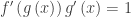
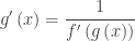
, then the point (b, a) is on the function’s inverse and the derivative here is \displaystyle \frac{1}{{f}'\left( a \right)}. This is just what my least favorite formula says: if f -1 (x) = g(x), then a = g(b)  and
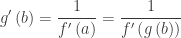
  \displaystyle {g}'\left( b \right)=\frac{1}{{f}'\left( a \right)}=\frac{1}{{f}'\left( g\left( b \right) \right)}.

What you really need to know is:

At corresponding points on a function and its inverse, the derivatives are reciprocals of each other.

This is what my least favorite formula says.

The AP exams have a clever way of testing this. (The stem may give a few more values to throw you off, or the values may be in a table.)

Given that f\left( 2 \right)=5\text{ and }{f}'\left( 2 \right)=3 and g is the inverse of f, Find {g}'\left( 5 \right).

The solution is reasoned this way: (5, ?) is a point on g. The corresponding point on f is (?, 5) = (2, 5). The derivative of f at this point is 3, therefore the derivative at (5, 2) on g is  {g}'\left( 5 \right)=\tfrac{1}{3}.

Easy!


Open or Closed?

About this time of year you find someone, hopefully one of your students, asking, “If I’m finding where a function is increasing, is the interval open or closed?”

Do you have an answer?

This is a good time to teach some things about definitions and theorems.

The place to start is to ask what it means for a function to be increasing. Here is the definition:

A function is increasing on an interval if, and only if, for all (any, every) pairs of numbers x1 < x2 in the interval, f(x1) < f(x2).

(For decreasing on an interval, the second inequality changes to f(x1) > f(x2). All of what follows applies to decreasing with obvious changes in the wording.)

  1. Notice that functions increase or decrease on intervals, not at individual points. We will come back to this in a minute.
  2. Numerically, this means that for every possible pair of points, the one with the larger x-value always produces a larger function value.
  3. Graphically, this means that as you move to the right along the graph, the graph is going up.
  4. Analytically, this means that we can prove the inequality in the definition.

For an example of this last point consider the function f(x) = x2. Let x2 = x1 + h where h > 0. Then in order for  f(x1) < f(x2) it must be true that

{{x}_{1}}^{2}<{{\left( {{x}_{1}}+h \right)}^{2}}
0<{{\left( {{x}_{1}}+h \right)}^{2}}-{{x}_{1}}^{2}
0<{{x}_{1}}^{2}+2h{{x}_{1}}+{{h}^{2}}-{{x}_{1}}^{2}
0<h\left( 2{{x}_{1}}+h \right)

This can only be true if {{x}_{1}}\ge 0, Thus, x2 is increasing only if x\ge 0.

Now, of course, we rarely, if ever, go to all that trouble. And it is even more trouble for a function that increases on several intervals.  The usual way of finding where a function is increasing is to look at its derivative.

Notice that the expression {{\left( {{x}_{1}}+h \right)}^{2}}-{{x}_{1}}^{2} looks a lot like the numerator of the original limit definition of the derivative of x2 at x = x1, namely \displaystyle {f}'\left( {{x}_{1}} \right)=\underset{h\to 0}{\mathop{\lim }}\,\frac{{{\left( {{x}_{1}}+h \right)}^{2}}-{{x}_{1}}^{2}}{h}. If h > 0, where the function is increasing the numerator is positive and the derivative is positive also. Turning this around we have a theorem that says, If {f}'\left( x \right)>0 for all x in an interval, then the function is increasing on the interval. That makes it much easier to find where a function is increasing: we simplify find where its derivative is positive.

There is only a slight problem in that the theorem does not say what happens if the derivative is zero somewhere on the interval. If that is the case, we must go back to the definition of increasing on an interval or use some other method. For example, the function x3 is increasing everywhere, even though its derivative at the origin is zero.

Let’s consider another example. The function sin(x) is increasing on the interval \left[ -\tfrac{\pi }{2},\tfrac{\pi }{2} \right] (among others) and decreasing on \left[ \tfrac{\pi }{2},\tfrac{3\pi }{2} \right]. It bothers some that \tfrac{\pi }{2} is in both intervals and that the derivative of the function is zero at x = \tfrac{\pi }{2}. This is not a problem. Sin(\tfrac{\pi }{2}) is larger than all the other values is both intervals, so by the definition, and not the theorem, the intervals are correct.

It is generally true that if a function is continuous on the closed interval [a,b] and increasing on the open interval (a,b) then it must be increasing on the closed interval [a,b] as well. (There is a proof by Lou Talman of this fact click here .)

Returning to the first point above: functions increase or decrease on intervals not at points. You do find questions in books and on tests that ask, “Is the function increasing at x = a.” The best answer is to humor them and answer depending on the value of the derivative at that point. Since the derivative is a limit as h approaches zero, the function must be defined on some interval around x = a in which h is approaching zero. So answer according to the value of the derivative on that interval.

You can find more on this here.

Case Closed.

Far Out!

A monster problem for Halloween.

A while ago I suggested you look at \displaystyle \underset{x\to \infty }{\mathop{\lim }}\,\frac{\ln \left( {{x}^{5}} \right)}{{{x}^{0.02}}} , which using the dominance idea is zero. Of course your students may try graphing or a table. Here’s the graph done by a TI-Nspire CAS. Note the scales.

This is not the way to go. Since the function is increasing near the origin, but the limit at infinity is zero there must be a maximum point where the function starts decreasing. And as the expression can never be negative once x > 1, there must be a point of inflection where the graph becomes concave up and can thereafter approach the x-axis from above as a horizontal asymptote. The maximum can be found by hand which makes for some great algebra manipulation practice:

\displaystyle \frac{d}{dx}\left( \frac{\ln \left( {{x}^{5}} \right)}{{{x}^{0.02}}} \right)=\frac{{{x}^{0.02}}\tfrac{5{{x}^{4}}}{{{x}^{5}}}-\ln \left( {{x}^{5}} \right)\left( 0.02{{x}^{-0.98}} \right)}{{{x}^{0.04}}}

\displaystyle \frac{d}{dx}\left( \frac{\ln \left( {{x}^{5}} \right)}{{{x}^{0.02}}} \right)=\frac{{{x}^{-0.98}}\left( 5-\left( 0.10 \right)\ln \left( x \right) \right)}{{{x}^{0.04}}}=\frac{50-\ln \left( x \right)}{10{{x}^{1.02}}}

Setting this equal to zero and solving gives x={{e}^{50}}\approx 5.185\times {{10}^{21}}

The second derivative is \displaystyle \frac{{{d}^{2}}}{d{{x}^{2}}}\left( \frac{\ln \left( {{x}^{5}} \right)}{{{x}^{0.02}}} \right)=\frac{-510+10.2\ln \left( x \right)}{100{{x}^{2.02}}}

and is zero when x\displaystyle {{e}^{\frac{520}{10.2}}}\approx 1.382\times {{10}^{22}}

Okay, I skipped a few steps here, but you can challenge your students with that. Since we’re really interested in the solution here more than the solving ,this is really a good place to use a CAS calculator.

The first line in the figure above defines the function to save typing it each time. The second line finds the x-coordinate of the maximum point (how do we know this is a maximum?) and the third finds the x-coordinate of the point of inflection.  Much simpler this way!

Take a minute to consider the numbers. They are BIG! In fact, if the units on our graph paper are centimeters, then the maximum point is a little over 5,480 light-years away from the origin! The point of inflection is about 2.665 times farther at more than 14,607 light-years away!

Meanwhile the maximum value is only 91.9699 cm. That’s right centimeters, less than a meter. And the y-coordinate of the point of inflection is about 91.9524 cm. A drop of 0.0175 cm. in a horizontal distance of a little over 9,127 light-years.

Some problems are a lot less scary if done with technology.