Introducing Power Series 1

The next few posts will discuss a way to introduce Taylor and Maclaurin series to students. We will kind of sneak up on the idea without mentioning where we are going or using any special terms. In this post we will find a way of approximating a function with a polynomial of any degree we choose. In the next post we will look at the graph of these polynomials and finally suggest some questions for further thought.

Making Better Approximations

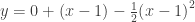
Students already know and have been working with the tangent line approximation of a function at a point (a, f(a)):

$f(x)\approx f\left( a \right)+{f}'\left( a \right)\left( x-a \right)$

ln(x):

For the function $f\left( x \right)=\ln \left( x \right)$ at the point (1, 0) ask your students to write the tangent line approximation: $y=0+(1)(x-1)$ .Point out that this line has the same value as ln(x) and its derivative as at (1, 0).

Then suggest that maybe having a polynomial that has the same value, first derivative and second derivative might be a better approximation. Suggest they start with $y=a+b\left( x-1 \right)+c{{\left( x-1 \right)}^{2}}$ and see if they can find values of a, b and c that will make this happen.

Since $f\left( 1 \right)=0,{f}'\left( 1 \right)=1\text{ and }{{f}'}'\left( x \right)=-1$ we can write

$y=a+b\left( x-1 \right)+c{{\left( x-1 \right)}^{2}};\quad y\left( 1 \right)=a+0+0=0;\quad a=0$

${y}'=b+2c\left( x-1 \right);\quad {y}'\left( 1 \right)=b+0=\tfrac{1}{1};\quad b=1$

${{y}'}'=2c;\quad {{y}'}'\left( 1 \right)=c=-\tfrac{1}{{{1}^{2}}}=-1;\quad c=-\tfrac{1}{2}$

$y=0+\left( x-1 \right)-\tfrac{1}{2}{{\left( x-1 \right)}^{2}}$

Then suggest they try a third degree polynomial starting with $y=a+b\left( x-1 \right)+c{{\left( x-1 \right)}^{2}}+d{{\left( x-1 \right)}^{3}}$ . Proceeding as above, all the numbers come out the same and we find that

$\ln \left( x \right)\approx 0+\left( x-1 \right)+\left( -\tfrac{1}{2} \right){{\left( x-1 \right)}^{2}}+\left( \tfrac{1}{3} \right){{\left( x-1 \right)}^{3}}$

Then go for a fourth- and fifth-degree polynomial until they discover the patterns. (The signs alternate, and the denominators are the factorial of the exponent.)

See if the class can write a general polynomial of degree N :

$\displaystyle \ln \left( x \right)\approx \sum\limits_{k=1}^{N}{\frac{{{\left( -1 \right)}^{k+1}}}{k}{{\left( x-1 \right)}^{k}}}$

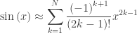
sin(x):

Then have the class repeat all this for a new function such as $f\left( x \right)=\sin \left( x \right)$ at the point (0, 0). This could be assigned as homework or group work. Ask them to do enough terms until they see the pattern. There will be patterns similar to ln(x ) and every other term (the even powers) will have a coefficient of zero.

$\sin \left( x \right)\approx x-\tfrac{1}{3!}{{x}^{3}}+\tfrac{1}{5!}{{x}^{5}}-\tfrac{1}{7!}{{x}^{7}}+\tfrac{1}{9!}{{x}^{9}}$

or in general the polynomial of degree N is

$\displaystyle \sin \left( x \right)\approx \sum\limits_{k=1}^{N}{\frac{{{\left( -1 \right)}^{k+1}}}{\left( 2k-1 \right)!}{{x}^{2k-1}}}$

How good is this approximation? Using only the first three terms of the polynomial above you will tell you that. Pretty close: correct to 5 decimal places. Using four terms gives correct to 7 decimal places when rounded.

Finally, see if they can generalize this idea to any function f at any point on the function $\left( {{x}_{0}},f\left( {{x}_{0}} \right) \right)$ . This time you will not have the various derivatives as numbers, rather they will be expressions like . Work through the powers one at a time to go from $y=a+b\left( x-{{x}_{0}} \right)+c{{\left( x-{{x}_{0}} \right)}^{2}}+d{{\left( x-{{x}_{0}} \right)}^{3}}+e{{\left( x-{{x}_{0}} \right)}^{4}}$

and so on, until you get to

$f\left( x \right)\approx f\left( {{x}_{0}} \right)+\frac{{f}'\left( {{x}_{0}} \right)}{1!}\left( x-{{x}_{0}} \right)+\frac{{{f}'}'\left( {{x}_{0}} \right)}{2!}{{\left( x-{{x}_{0}} \right)}^{2}}$

$\quad \quad \quad \quad \quad \quad \quad \quad \quad \quad \quad \quad \quad +\cdots +\frac{{{f}^{\left( N \right)}}\left( {{x}_{0}} \right)}{N!}{{\left( x-{{x}_{0}} \right)}^{N}}$

For example the third derivative computation would look like this:

${{{y}'}'}'=3\cdot 2\cdot 1d+4\cdot 3\cdot 2e\left( x-{{x}_{0}} \right)$

${{{y}'}'}'\left( {{x}_{0}} \right)=3\cdot 2\cdot 1d+4\cdot 3\cdot 2e(0)={{{f}'}'}'\left( {{x}_{0}} \right)$

$d=\frac{{{{f}'}'}'\left( {{x}_{0}} \right)}{3!}$

The computations here are perhaps a little different than what students have seen, so take your time doing this. Two or even three class days may be necessary.

Notice these things:

The first two terms are the tangent line approximation.
The various derivatives are numbers that must be calculated.
All the terms of any degree are the same as the terms of the previous degree with one additional term.

Next post in this series: Looking at all this graphically.

(Typos in an earlier version of this post have been corrected – LMc)

2 thoughts on “Introducing Power Series 1”

SL on February 1, 2015 at 23:46 said:

Lin –
Taught AB for years, but this is my first go with BC. Anxious for series as I remember this being where the wheels fell off for me as a student. I’m been hammering tangent lines this year, and we recently did Euler’s Method where we adapted the typical point-slope format for y=y_1 + m(x-x_1). Think with that launching point, this structure will be well worth my time to use in class. Appreciate the ideas.

LikeLike

Reply ↓
mrdardy on February 9, 2013 at 10:57 said:

Lin

Thanks for this post. Just about ready to dive into this with my BC gang this week and this will help me unpack this all.

LikeLike

Reply ↓

Teaching Calculus

The pleasure lies not in discovering the truth, but in searching for it.

Introducing Power Series 1

2 thoughts on “Introducing Power Series 1”

Leave a Reply Cancel reply

Share this:

Like this:

Related

2 thoughts on “Introducing Power Series 1”

Leave a Reply Cancel reply