Good Question 9

This is a good question that leads to other good questions, both mathematical and philosophical. A few days ago this question was posted on a private Facebook page for AP Calculus Readers. The problem and illustration were photographed from an un-cited textbook.

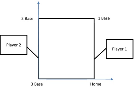
Player 1 runs to first base [from home plate] at a speed of 20 ft/s while player 2 runs from second base to third base a speed of 15 ft/s. Let s be the distance between the two players. How fast is s changing when player 1 is 30 feet from home plate and Player 2 is 60 feet from second base. [A figure was given showing that the distance between the bases is 90 feet.]

baserunners 2-8-16

Some commenters indicated some possible inconsistencies in the question, such as assuming the Player 2 is on second base when Player 1 leaves home plate. In this case the numbers don’t make sense. So, someone suggested this must be a hit-and-run situation. To which someone else replied that with a lead of that much it’s really a stolen base situation. So, the first thing to be learned here is that even writing a simple problem like this you need to take some of the real aspects into consideration. But this doesn’t change the mathematical aspects of the problem.

One of the things I noticed before I attempted to work out the solution was that Player 2 is the same distance from third base as Player 1 is from home plate. I verbalized this as “players are directly across the field from each other.” I filed this away since it didn’t seem to matter much. Wrong!

Then I worked on the problem two ways. These are shown in the appendix at the end of this post. I discovered (twice) that s’ = 0; at the moment suggested in the question the distance is not changing.

Then it hit me. Doh! – I didn’t have to do all that. So, I posted this solution (which I now notice someone beat me to):

At the time described, the players are directly across the field from each other (90 feet apart). This is the closest they come. The distance between them has been decreasing and now starts to increase. So, at this instant s is not changing (s‘ = 0).

The Philosophical Question

Then the original poster asked for someone “to post [actual] work done in calculus” and “to see some related rates.” So, I posted some “calculus” and got to thinking – the philosophical question – isn’t my first answer calculus?

I think it is. It makes use of an important calculus concept, namely that as things change, at the minimum place, the derivative is zero. Furthermore, the justification (that the distance changes from decreasing to increasing at the minimum implies the derivative is zero) is included. * Why do you need variables?

Also, this solution is approached as an extreme value (max/min) problem rather than a related rate problem. This shows a nice connection between the two types of problems.

The Related (but not related rate) Good Question

So here is another calculus question with none of the numbers we’ve grown to expect:

Two cars travel on parallel roads. The roads are w feet apart. At what rate does the distance between the cars change when the cars are w feet apart?

Notice:

  • That the cars could be travelling in the same or opposite directions.
  • Their speeds are not given.
  • You don’t know when or where they started; only that at some time they are opposite each other (w feet apart).
  • In fact, they could start opposite each other and travel in the same direction at the same speed, remaining always w feet apart.
  • One car could be standing still and the other just passes it.

But you can still answer the question.

(*Continuity and differentiability are given (or at least implied) in the original statement of the problem.)

 Appendix

My first attempt was to set up a coordinate system with the origin at third base as shown below.

Blog 2-8-16

Then, taking the time indicated in the problem as t = 0, the position of Player 1 is (90, 30 + 20t) and the position of player 2 is (0, 30 – 15t). Then the distance between them is

s=\sqrt{{{90}^{2}}+{{\left( 30-15t-\left( 30+20t \right) \right)}^{2}}}=\sqrt{{{90}^{2}}+{{\left( -35t \right)}^{2}}}

and then

\displaystyle {s}'\left( t \right)=\frac{2\left( -35t \right)\left( -35 \right)}{2s}\text{ and }{s}'\left( 0 \right)=0

This is correct, but for some reason I was suspicious probably because zeros can hide things. So I re-stated this time taking t = 0 to be one second before the situation described in the problem. Now player 1’s position is (90, 10+20t) and player 2’s position is (0, 45-15t).

s\left( t \right)=\sqrt{{{90}^{2}}+{{\left( 45-15t-\left( 10+20t \right) \right)}^{2}}}=\sqrt{{{90}^{2}}+{{\left( 30-35t \right)}^{2}}}

\displaystyle {s}'\left( t \right)=\frac{2\left( 35-35t \right)\left( -35 \right)}{2s}\text{ and }{s}'\left( 1 \right)=0

.

____________________________________________

Trapezoids – Ancient and Modern

The other day, in the course of about 10 minutes, I came across two interesting things about Trapezoidal approximations that I thought I would share with you.

cuneifirm tablet

Cuneiform writing

The first was a link to a story about how the ancient Babylonian astronomers sometime between 350 and 50 BCE used trapezoids to, in effect, find the area under a velocity-time graph tracking Jupiter’s motion. This was an NPR story based on a January 2016 Science magazine article in which the author, Mathieu Ossendrijver discusses his work deciphering cuneiform tablets written over 1,400 years before the technique showed up in Europe.


The second was a question asked on the AP Calculus bulletin board. A teacher asked, “Can someone please help me answer this question a student posed the other day. We were comparing left, right and midpoint and trapezoidal approximations. He asked since the trapezoidal calculation is the best estimate what is the use of LRAM and RRAM?” Here is an expanded form of my answer.

There are several things to consider here.

  1. First, if all you need is an estimate of the area or integral of a continuous function then a Trapezoid sum is certainly better than the left Riemann sum (left-RΣ) or the right-RΣ. Better, yes, the “best” maybe not: midpoint sums are about as good and parabola sums (Simpson’s Rule) are better.

2. Another reason to do left RΣ and right RΣ with small values of n is simply to give students practice in setting up Riemann sums so that they will be familiar with them when they move on to finding their limits and getting ready to define definite integrals.

3. A RΣ for a function f on a closed interval [a, b] is formed by partitioning the interval into subintervals and taking exactly one function value from each closed subinterval, multiplying the value by the width of that subinterval and adding these results. You may pick the function value any way you want – left end, middle, right end, any place at random in the subintervals and someplace else in the next subinterval. One way is to pick the smallest function value in each subinterval; this gives a RΣ called the lower RΣ. Likewise, you could pick the largest value in each subinterval; this gives the upper RΣ. Now it is true that

lower RΣ ≤ (any/all other RΣs) ≤ upper RΣ

Then as you add more partition points (n approaches infinity, or Δx approaches 0, etc.) the lower sum increases and the upper sum decreases. The series of lower sums is increasing and bounded above (by the upper sum) and therefore converges to its least upper bound. The upper sum decreases forming a decreasing series that is bounded below and therefore converges to its greatest lower bound.

If the lower RΣ and the upper RΣ approach the same value, then ALL the other RΣs approach that same value by the Squeeze theorem. This value is then defined as the definite integral of f from a to b.

In most AP calculus course, the textbooks do not deal with upper and lower sums. Instead, they deal with left RΣ and right RΣ on intervals on which f is only increasing (or only decreasing). In this case the lower RΣ = left RΣ and the upper RΣ = the right RΣ (or the other way around for decreasing functions).

So, this is why you need the left RΣ and right RΣ; not so much to approximate, but to complete the theory leading to the definite integral.

February 2016

As I hope you’ve noticed there is a new pull-down on the navigation bar called “Website.” For some years I’ve had a website at linmcmullin.net that lately I’ve been neglecting. I decided to close it in the next few days, and therefore, I move most of the material that is there to this new tab. The main items of interest are probably those under “Calculus”, “Winplot”, and “CAS.” If you used that website you should be able to find what you need here. If you cannot find something, then please write and I’ll try to help.

In my post entitled January 2016 are listing of post for the applications of integration for both AB and BC calculus. This month’s posts are BC topics on sequences, series, and parametric and polar equations.

Posts from past Februarys

Sequences and Series

February 9, 2015 Amortization A practical application of sequences.

February 8, 2013: Introducing Power Series 1

February 11, 2013: Introducing Power Series 2

February 13, 2013: Introducing Power Series 3

February 15, 2013 New Series from Old 1

February 18, 2013: New Series from Old 2

February 20, 2013: New Series from Old 3

February 22, 2013: Error Bounds

May 20, 2015 The Lagrange Highway

Polar, Parametric, and Vector Equations

March 15, 2013 Parametric and Vector Equations

March 18, 2013 Polar Curves

May 17, 2014 Implicit Differentiation of Parametric Equations 

A series on ROULETTES some special parametric curves (BC topic – enrichment):


What’s Your Favorite?

A very short post today. Audrey Weeks, author of Calculus in Motion, sent me this link to a BBC article by Melissa Hogenboom discussing the 10 most beautiful equations. Each equation can be clicked for more details and some of the links even have videos discussing the equation. Click here for You decide: What is the most beautiful equation? After reading about them, you can vote for your favorite and see the results so far.

beautiful equations

Good Question 8 – or not?

Seattle rainToday’s question is not a good question. It’s a bad question.

But sometimes a bad question can become a good one.

This one leads first to a discussion of units, then to all sorts of calculus.

Here’s the question a teacher sent me this week taken from his textbook:

The normal monthly rainfall at the Seattle-Tacoma airport can be approximated by the model R=3.121+2.399\sin \left( 0.524t+1.377 \right), where R is measured in inches and t is the time in months, t = 1 being January. Use integration to approximate the normal annual rainfall.  Hint: Integrate over the interval [0,12].

Of course, with the hint it’s not difficult to know what to do and that makes it less than a good question right there. The answer is \displaystyle \int_{0}^{12}{R(t)dt=37.4736} 
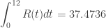
inches. You could quit here and go on to the next question, but …

Then a student asked. “If R is in inches shouldn’t be in units of the integral be inch-months, since the unit of an integral is the unit of the integrand times the units of the independent variable?”  Well, yes, they should. So, what’s up with that?

Also, the teacher figured that the integral of a rate is an amount and our answer is an amount, so why isn’t the integrand a rate?

The only answer I could come up with is that the statement “R is measured in inches” is incorrect; R should be measured in inches /month. The opening phrase “normal monthly rainfall” also seems to point to the correct units for R being inches/month.

Problem solved; or maybe does this lead to a different concern?

The teacher pointed out that R(6) = 0.7658 inches is a reasonable answer for the amount of rain in June whereas \displaystyle \int_{0}^{6}{R(t)dt=}20.4786 is not.

If R is a rate, then the amount of rain that falls in June (t = 6) is given by \displaystyle \int_{5}^{6}{R(t)dt}=0.9890.

From here on we will assume that R is a rate with units of inches/month. Here are the individual monthly rates calculated with a CAS. Ques 8 a

The total amount of rainfall (second line above) appears be R(1) + R(2) + R(3) + … +R(12) = 37.4742. This is very close to the amount calculated by integration.

The slight difference of 0.0006 is not a round off error.

Remember, behind every definite integral there is a Riemann sum!

Again, the units are the problem. Why does the sum of the monthly rates seem to give the total amount?  The reason is that the terms of the sequence above are actually the values of a right-side Riemann sum of the rate, R(t), over the interval [0,12] with 12 equal subdivisions of width 1 (month) each with the 1’s left out as 1’s often are. Therefore, their sum should come close to the total yearly rainfall, but it is really just an approximation of it.

The actual total for any month, n, is given by \displaystyle \int_{n-1}^{n}{r(t)}dt
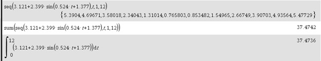
. For example the amount of rain that falls in June is given by \displaystyle \int_{5}^{6}{R(t)dt}=0.9890 inches.

Here is the sequence of the actual monthly rainfall values in inches, and their sum.

Ques 8 b

This agrees with the integral. Why? Because one of  the properties of integrals tell us that \displaystyle \sum\limits_{n=1}^{12}{\int_{n-1}^{n}{r(t)dt}}=\int_{0}^{12}{r(t)dt}.


Another instructive thing with this integral is this: The function R=3.121+2.399\sin \left( 0.524t+1.377 \right) is periodic with a period of  \frac{2\pi }{0.524}\approx 11.9908\approx 12. So the sine function takes on (almost) all its values in a year, as you would expect. Since the sine values all but cancel each other out

\displaystyle \int_{0}^{12}{3.121+2.399\sin \left( 0.524t+1.377 \right)dt}\approx \int_{0}^{12}{3.121dt=3.121\left( 12-0 \right)=37.452}. Close!

The total rainfall divided by 12 is \frac{37.452}{12}=3.121 this must be close to the average rainfall each month. The average rainfall is \displaystyle \frac{1}{12}\int_{0}^{12}{R\left( t \right)dt}=3.1228 inches. Close, again!


So, there you have it. Is this a good question or not? We considered all these concepts while working not just with an equation but with numbers from a poorly stated problem:

  • Reading and interpreting words.
  • Unit analysis
  • Integration by technology
  • Realizing that a pretty good approximation is not correct, due again to units.
  • A Riemann sum approximation in a real situation that comes very close to the value by integration
  • Using a property of a periodic function to greatly simplify an integral
  • Finding average value two ways

So, it turned out to be a sunny day in Seattle.seattle sun

.

January 2016

HAPPY NEW YEAR

– a few more days off and then back to school!

If you haven’t already, it is time to start integration. The posts on starting integration were listed in December since I try to stay ahead of things so you’ll have time to prepare. With that in mind here are past posts on applications of integration – area, volume, average value, improper integrals, accumulation, and some enrichment for BC classes on parametric equations. This will take AB courses well into February. The February postings will be for the BC topics on sequences and series.

The four featured post below are the most popular from this list.

Applications of integration: area, volume, average value of a function, Accumulation and functions defined by integrals.

January 2, 2013 Integration by Parts – 1

January 4, 2013 Integration by Parts – 2

January 7, 2013 Area Between Curves

 A series on visualizing solid figures:Solid rotation

January 9, 2013 Volume of Solids with Regular Cross-sections

January 11, 2013 Volumes of Revolution

January 14, 2013 Why You Never Need Cylindrical Shells

January 25, 2014 Improper Integrals and proper areas.

January 16, 2013 Average Value of a Function

February 6, 2013: Logarithms

January 19, 2013 Most Triangles are Obtuse! What is the probability that a triangle picked at random will be acute? An average value problem solved by a tenth grader.

 A series on ROULETTES some special parametric curves (BC topic – enrichment):

Accumulation – On the exams; not in many textbooks 

.

When are we ever …?

Allen Wohlmer

The following answer to a question we’ve all been asked was posted yesterday on a private Facebook page for AP Calculus readers. The author, Allen Wolmer is a teacher and AP Calculus reader. He teaches at Yeshiva Atlanta High School, in Atlanta, Georgia. I reprint it here with his kind permission.

Thank you, Allen.


A colleague of mine teaching high school math asked me the following:

“So some of my kids are struggling with the math concepts and ideas (why do I need to learn this? When will I ever use factoring/polynomials?). I would say most of my students have not had a particularly good relationship with math in the past.

I have answered these questions, with responses like financial jobs, accounting, econ, but they have no interest in these types of jobs/real world applications.

I have also talked about logic, problem solving, and puzzles.
Do you have any advice for me, and or ideas to share with them?”

Here is my reply:

“Glad to help.
First of all, recognize that, for the most part, the kids aren’t really interested in your answer. They are just being lazy and looking for a reason, any reason, to not do work, any work.
Now, how do you answer? Well, you can try the face value approach, that is describing engineering, actuary, etc., but that will be meaningful to just a handful of students, and they’re not the ones asking the question anyway.

So, I turn it around. I ask the boys how many go the gym or health club or weight room to work out. Hands quickly shoot up (after all, they want to be cool in front of their buds and the chicks). I then ask them how many use the pec machine (it’s the one where you raise your arms to shoulder level and bring the elbows together). I demonstrate with the motion. Many of them admit they use the machine. I then ask them when they would ever use that motion in real life. The answer, of course, is NEVER! So, why do you do it, I ask them. I answer for them “because it strengthens your muscles!”

And that’s why we study mathematics: to strengthen our mental muscles. We’re not really studying math, I tell them. We’re studying how to analyze and understand problems when we read them. What do we know? What do we not know? What are we trying to find?

We’re learning how to pay attention to detail. We’re learning how to be precise in our thinking and our work. We’re learning how to be neat in our work. We’re learning to look for patterns. We’re learning to look for similarities to other problems we have solved. We’re learning how to look at our results and determine if they make sense or not.
In other words, we’re learning how to think critically and solve problems. We’re doing it in the context of learning mathematics, but that’s only because that’s the best environment to do it in.

Then I tell them never to ask that #$%^%$# question again and to shut the #$%^&*&^% up and get back to work!

Sincerely,
Allen Wolmer”

.