Concepts Related to Graphs

This and the next several posts will be about graphing and specifically how the function and its first and second derivatives are related. Since I do not intend this to be a textbook, I will not be doing textbook stuff. Rather, I hope to add some big picture things about the concepts involved. Hope you find it useful.

________________________________

Graphs of functions come in some combination of five shapes:

• Linear,
• Increasing, concave up,
• Increasing, concave down,
• Decreasing, concave up, and
• Decreasing, concave down.

I have put together an activity, An Exploration of the Shape of a Graph, to help students learn the relationship between the shapes and the derivative. Leaving the linear sections aside, the idea of the activity is to call students’ attention to the other four shapes and the slope of the tangent line (the derivative) in the intervals where the graph has each shape.

The key is to keep focused on the tangent line. To this end I suggest drawing short tangent segments parallel to the graph, as illustrated in the figure below.

Air-graphing: Another way to help students internalize this idea is to draw the graph of a function on the board and then have the students hold their pen out in front of them so the pen looks like a segment tangent to the graph. Then move the pen along the graph paying attention to the slope.

Either way what you want students to be aware of is

(1) Where the slopes are positive and where they are negative. This will later be related to the intervals where the function increases and decreases, and

(2) How the slope itself is changing. Is the slope increasing or decreasing? This will later be related to the concavity.

I hope you and your students find this activity helpful.

Why Radians?

Calculus is always done in radian measure. Degree (a right angle is 90 degrees) and gradian measure (a right angle is 100 grads) have their uses. Outside of the calculus they may be easier to use than radians. However, they are somewhat arbitrary. Why 90 or 100 for a right angle? Why not 10 or 217?

Radians make it possible to relate a linear measure and an angle measure. A unit circle is a circle whose radius is one unit. The one-unit radius is the same as one unit along the circumference. Wrap a number line counterclockwise around a unit circle starting with zero at (1, 0). The length of the arc subtended by the central angle becomes the radian measure of the angle.

This keeps all the important numbers like the sine and cosine of the central angle, on the same scale. When you graph y = sin(x) one unit in the x-direction is the same as one unit in the y-direction. When graphing using degrees, the vertical scale must be stretched a lot to even see that the graph goes up and down. Try graphing on a calculator y = sin(x) in degree mode in a square window and you will see what I mean.

But the utility of radian measure is even more obvious in calculus. To develop the derivative of the sine function you first work with this inequality (At the request of a reader I have added an explanation of this inequality at the end of the post):

\displaystyle \frac{1}{2}\cos \left( \theta \right)\sin \left( \theta \right)\le \frac{1}{2}\theta \le \frac{1}{2}\tan \left( \theta \right)

From this inequality you determine that \displaystyle \underset{\theta \to 0}{\mathop{\lim }}\,\frac{\sin \left( \theta \right)}{\theta }=1

The middle term of the inequality is the area of a sector of a unit circle with central angles of \theta 
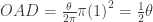
radians. If you work in degrees, this sector’s area is \displaystyle \frac{\pi }{360}\theta  and you will find that
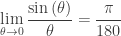
 \displaystyle \underset{\theta \to 0}{\mathop{\lim }}\,\frac{\sin \left( \theta \right)}{\theta }=\frac{\pi }{180}.

This limit is used to find the derivative of the sin(x). Thus, with x in degrees, \displaystyle \frac{d}{dx}\sin \left( x \right)=\frac{\pi }{180}\cos \left( x \right)
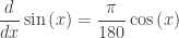
. This means that with the derivative or antiderivative of any trigonometric function that \displaystyle \frac{\pi }{180} is there getting in the way.

Who needs that?

Do your calculus in radians.


Revision December 7, 2014: The inequality above is derived this way. Consider the unit circle shown below.

unit circle

1. The central angle is \theta  and the coordinates of A are \left( \cos (\theta ),\sin (\theta ) \right).

Then the area of triangle OAB is \frac{1}{2}\cos \left( \theta\right)\sin \left( \theta\right)

2. The area of sector OAD=\frac{\theta}{2\pi }\pi {{\left( 1 \right)}^{2}}=\frac{1}{2}\theta 
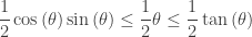
. The sector’s area is larger than the area of triangle OAB.
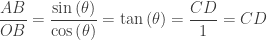
3. By similar triangles \displaystyle \frac{AB}{OB}=\frac{\sin \left( \theta\right)}{\cos \left( \theta\right)}=\tan \left( \theta\right)=\frac{CD}{1}=CD.

Then the area of \Delta OCD=\frac{1}{2}CD\cdot OD=\frac{1}{2}\tan \left( \theta \right) This is larger than the area of the sector, which establishes the inequality above.

Multiply the inequality by \displaystyle \frac{2}{\sin \left( \theta \right)} and take the reciprocal to obtain
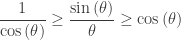
 \displaystyle \frac{1}{\cos \left( \theta \right)}\ge \frac{\sin \left( \theta \right)}{\theta }\ge \cos \left( \theta \right).

Finally, take the limit of these expression as \theta \to 0 and the limit \displaystyle \underset{\theta \to 0}{\mathop{\lim }}\,\frac{\sin \left( \theta \right)}{\theta }=1 is established by the squeeze theorem.

Related Rate Problems II

If you look in most textbooks for related rate questions you will find pretty much the same related rate problems: ladders sliding down walls, people walking away from lamppost, water running into or out of cone shaped tanks, etc.

Here are two somewhat different related problems you may like.

  1. A girl starts riding down an escalator at the same time a boy starts riding up a parallel escalator. The escalators are 5 meters apart, 30 meters long, and they both move at the rate of 1 m/sec.
    1. How fast is the distance between the kids changing 10 seconds later? (Answer: -1.789 m/sec.)
    2. Variation: Suppose that the girl is moving at 1 m/sec and the boy at 3 m/sec. The boy reaches the end of the escalator first and stands there. Now how fast is the distance between them changing 8 seconds after they start?  (1.486 m/sec)
    3. Variation: With the situation given in part b., write and graph a piece-wise defined function that gives the distance between the kids.  Find where this graph is continuous but not differentiable. Why does this happen? (Answer: the boy reaches the top in 10 seconds and stands still. Up to this point the distance between them is represented by a hyperbola; here it now becomes a different parabola with an abrupt change in the graph. At this point, the function is not differentiable. This second parabola appears almost linear from the 10 second point on.
  1. A 60-foot-long rope is attached to a pulley 36 feet above the ground. A lantern his attached to one end of the rope and a man holds the other end on the top of his head 6 feet off the ground. He walks away at the rate of 5 feet/sec.
    1. Find the rate at which the distance between the pulley and the top of the man’s head is changing when he is 40 feet from the point directly under the pulley? (Answer: 4 ft./sec.)
    2. Find the rate of change of the length of the man’s shadow when he is 40 feet from a point directly under the pulley? (Answer:  -0.90 ft./sec.)
    3. (Extension – extreme value problem, rather difficult) When the man starts walking the lantern is at the height of his head and his shadow is infinitely long. When is the tip of the man’s shadow closest to the point directly under the pulley and how far away is it? (Answer: At t = 3.654 sec the tip of the shadow is 39.658 feet from the point under the pulley.)

These two questions are from Audrey Weeks’ Calculus in Motion. This is a really good package of dynamic illustrations of calculus concepts and AP Exams free-response question that runs on Geometer’s Sketchpad. For more information click here. The related rate sections include both standard and non-standard problems.

Corrections made September 17, 2014, March 6, 2022

Related Rate Problems I

Related rate problems provide an early opportunity for students to use calculus in a more or less, real context and practice implicit differentiation.

One of the problems students have with these problems is that almost all of them involve writing the model or starting equation based on some geometric situation. Students must switch from calculus to geometry and then back again. When starting out, one of the ways to avoid this is to give a few problems that do not involve any geometry. Once they have the idea of relating the rates by using the derivative, then they may be ready to tackle the geometry.

Here are two examples of related rate problems without geometry (answers at the end).

1. The kinetic energy, K in joules, of a moving object is given by the equation K=\tfrac{1}{2}m{{v}^{2}} where m is the mass of the object and v is its velocity. The mass of a rocket decreases at a constant rate of 25 kg/sec due to the burning of its fuel. When the mass of the rocket is 6000 kg, the velocity is 12 m/sec and increases at the rate of 2 m/sec/sec. At this instant how fast is the kinetic energy in changing? (The units are joules / sec.)

2. The force, F in Newtons, of a moving object is given by the equation F=ma where m is the mass of the object and a is its acceleration. A rocket sled is propelled along a track with an acceleration given by a(t)=5{{t}^{2}}+6t\text{ for }t\ge 0. When t = 6 sec. its mass is 10 kg and is decreasing at the rate of 0.2 kg/sec due to the burning of its fuel. At this instant how fast is the force changing?

The next post will be two out of the ordinary related rate problems (with geometry).

Answers:  1. 142,200 joules / sec.  2.   616.8 Newtons / sec

Derivative Practice – Graphs

Another way to practice the derivative rules.

The graph below shows two piecewise defined functions, f and g, each consisting of two line segments.

  1. If h\left( x \right)=2g\left( x \right)-5f\left( x \right) calculate {h}'\left( 3 \right)
  2. If j\left( x \right)=f\left( x \right)g\left( x \right) calculate {j}'\left( -4 \right)
  3. If k\left( x \right)={{x}^{2}}f\left( x \right) calculate {k}'\left( 5 \right)
  4. If  r\left( x \right)=f\left( g\left( x \right) \right)  calculate {r}'\left( 0 \right)
  5. Write the equation of the line tangent to the graph of y=2+f\left( x \right)g\left( x \right) at the point  \left( -4,2 \right).

There are a lot more like these that you can ask from the same graph; or make up your own graph and questions.

Answers:  1. -17/3,     2. 6,     3.  75,     4. -1/3,     5. y = 2 + 6(x + 4)   (Corrected 10-3-12 19:10)

Derivative Practice – Numbers

Here is an example of how to help your students practice their derivative rules in a different way. Tomorrow another different approach.
Let f be a differentiable function. The table below gives values of f and g their first derivatives at selected values of x

x   -2    0   2   4   6
 f\left( x \right) -8 0 –2 2 5
 {f}'\left( x \right)  2  4 –3 –1 0
 g\left( x \right) 2 4 5 6 5
 {g}'\left( x \right) 1 2 4 3  2
    1. If h\left( x \right)=f\left( x \right)+3g\left( x \right) find  {h}'\left( 2 \right)
    2. If \displaystyle j\left( x \right)=\frac{f\left( x \right)}{g\left( x \right)} find  {j}'\left( 4 \right)
    3. If  r\left( x \right)=f\left( g\left( x \right) \right)  find  {r}'\left( 0 \right)
    4. If  s\left( x \right)=g\left( f\left( x \right) \right)  find  {s}'\left( 2 \right)
    5. If  q\left( x \right)=g\left( x \right)f\left( x \right) find  {q}'\left( -2 \right)
    6. Approximate  {g}'\left( 3 \right)
    7. Write an equation of the line tangent to g at the at the point where = 0.

Answers:

1. 9,     2. -1/3,     3. -2,     4. -3,     5. -5,     6. 1/2,    7.  y=4+2(x-0) or y = 4+2

The Mean Value Theorem II

The Rule of Four suggests that mathematics be studied from the analytical, graphical, numerical, and verbal points of view. Proof can only be done analytically – using symbols and equations. Graphs, numbers, and words aid in that, but do not by themselves prove anything.

On the other hand, numbers and especially graphs can make many of the theorems much more understandable and often can convince one of the truth of a theorem far better than the actual proof.

The Mean Value Theorem, MVT, is a good example; it can be demonstrated with a lot less trouble. See the figure above. Picture the blue line connecting the endpoints of the interval (the secant line) moving up, parallel to its original position. See the figure above. As this line moves up it intersects the graph twice, until eventually, just before it does not intersect at all, it comes to a place where it intersects exactly one. At this point it is tangent to the original graph. Since it is tangent, the slope of the line is the same as the derivative, {f}'\left( c \right), at that point.

So, the derivative is equal to the slope of the line between the endpoints. The MVT says that if its hypotheses are true, then there must be a place where the slope of the tangent line is parallel to the slope of the secant line.
But wait, there is more: at that point the instantaneous rate of change of the function is equal to the average rate of change over the interval.

This shows a real strength of looking at the graph.

But it is only one of many possible graphs. The graph could look like this figure:

Here there are several places (5 to be exact) where the tangent line is parallel to the secant line; there could be several on one side, or several on both sides. But this is not a problem; this does not contradict the MVT, which says there is at least one.

Yet another way to show the MVT is this. Near the left end of the first graph above the slope of the tangent to the graph (the derivative) is larger than the slope of the secant line; near the right end the slope of the tangent is less than the slope of the secant. So somewhere in between, by the Intermediate Value Theorem, the slope of the tangent must equal the slope of the secant. (For the purists out there, this is from Darboux’s theorem, and requires a slightly stronger hypothesis, namely that the one-sided derivatives at a and b exist.)

Rolle’s theorem can be demonstrated with either of these approaches as well. Rolle’s Theorem is really a special case of the MVT where the slope of the secant line is zero.

In conclusion, I think that this sequence of theorems is a good place to do a little proving of theorems. On the other hand you can easily show the results other ways. In fact, the method at the beginning of this post should be shown anyway in order to give students a good picture (no pun intended) of the MVT. It will help them remember what it is all about.