Graphing Integrals

Posted on November 15, 2016 by Lin McMullin

The sixth in the Graphing Calculator / Technology series

The topic of integration is coming up soon. Here are some notes and ideas about the integration operation on graphing calculators. The entries are the same or very similar for all calculator brands.

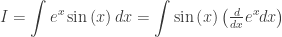
The basic problem of evaluating a definite integral on a graphing calculator is done without finding an antiderivative; that is, the calculator uses a numerical algorithm to produce the result. The calculator provides a template,and you fill in the 4 squares so that the expression looks exactly like what you write by hand. Then the calculator computes the result. (Older models require a one-line input requiring, in order, the integrand, the independent variable, the lower limit of integration and the upper limit in that order, separated by commas.) The first interesting thing is that the variable in the integrand does to have to be x. As the first figure illustrates using x or a or any other letter gives the same result.

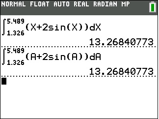
This is because the variable of integration is just a place holder. Sometimes called a “dummy variable”, this letter can be anything at all, including x. On the home or calculation screen you might as well always use x, so the entry will look like what you have on your paper. As we will see, when graphing it may be less confusing to use a different letter.

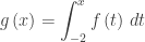
The antiderivative, F, of any function, f, can be written as a function defined by an integral where there is a point on the antiderivative of f , which is with F ’ = f. The point (a, F(a)) is the initial condition. (In the following we will use F(a) = 0 as the initial condition – the graph will contain the origin. As a further investigation, try changing the lower limit to different numbers and see how that changes the graph.)

The integration operation can be used to graph the antiderivative of a function without finding the antiderivative. You may graph the antiderivative when teaching antiderivatives. Have students look at the graph of the antiderivative and guess what that function is.

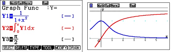
When graphing use x as the upper limit of integration and a different letter for the variable in the rest of the template. The calculator will use different values of x to calculate the points to be graphed.

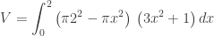
The set-up shown in the next figure shows how to enter a function defined by an integral (blue line) and the same function obtained by antidifferentiating (red squares). As you can see the results are the same.

In this way, you can explore the functions and their indefinite integrals by graphing.

The Fundamental Theorem of Calculus

Another use of using the graph of an integral is to investigate both parts of the Fundamental Theorem of Calculus (FTC). Roughly speaking, the FTC says that the integral of a derivative of a function is that function, and the derivative of an integral is the integrand.

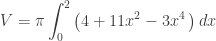
In the figure below, the same function is entered both ways; the graphs are the same. (Note the x’s in the second line must be x in all four places.)

Parts and More Parts

Posted on August 5, 2016 by Lin McMullin

At an APSI this summer the participants and I got to discussing the “tabular method” for integration by parts. Since we were getting far from what is tested on the BC Calculus exams, I ended the discussion and said for those that were interested I would post more on the tabular method this blog going farther than just the basic set up. So here goes.

Here are some previous posts on integration by parts and the tabular method

Integration by Parts 1 discusses the basics of the method. This is as far as a BC course needs to go.

Integration by Parts 2 introduces the tabular method

Modified Tabular Integration presents a very quick and slick way of doing the tabular method without making a table. This is worth knowing.

There is also a video on integration by parts here. Scroll down to “Antiderivatives 5: A BC topic – Integration by parts.” The tabular method is discussed starting about time 15:16. There are several ways of setting up the table; one is shown here and a slightly different way is in the Integration by Parts 2 post above. There are others.

Going further with the tabular method.

The tabular method works well if one of the factors in the original integrand is a polynomial; eventually its derivative will be zero and you are done. These are shown in the examples in the posts above and Example 1 below. To complete the topic, this post will show two other things that can happen when using integration by parts and the tabular method.

First we look at an example with a polynomial factor and learn how to stop midway through. Why stop? Because often there will be no end if you don’t stop. There are ways to complete the integration as shown in the examples.

Example 1: Find $\displaystyle \int_{{}}^{{}}{\left( 4{{x}^{3}} \right)\cos \left( x \right)dx}$ by the tabular method (See Integration by Parts 2 for more detail on how to set the table up)

Adding the last column gives the antiderivative:

$\displaystyle \int_{{}}^{{}}{\left( 4{{x}^{3}} \right)\cos \left( x \right)dx}=4{{x}^{3}}\sin \left( x \right)+12{{x}^{2}}\cos \left( x \right)-24x\sin \left( x \right)-24\sin \left( x \right)+C$

Now say you wanted to stop after $12{{x}^{2}}\cos \left( x \right)$ . Example 2 shows why you want (need) to stop. In Example 1 you will have

$\displaystyle \int_{{}}^{{}}{\left( 4{{x}^{3}} \right)\cos \left( x \right)dx}=4{{x}^{3}}\sin \left( x \right)+12{{x}^{2}}\sin \left( x \right)+\int_{{}}^{{}}{-24x\cos \left( x \right)}dx$

The integrand on the right is the product of the last column in the row at which you stopped and the first two columns in the next row, as shown in yellow above.

Example 2 Find $\displaystyle \int_{{}}^{{}}{{{e}^{x}}\cos \left( x \right)dx}$

As you can see things are just repeating the lines above sometimes with minus signs. However, if we stop on the third line we can write:

$\displaystyle \int_{{}}^{{}}{{{e}^{x}}\cos \left( x \right)dx={{e}^{x}}\sin \left( x \right)}+{{e}^{x}}\cos \left( x \right)-\int_{{}}^{{}}{{{e}^{x}}\cos \left( x \right)dx}$

The integral at the end is identical to the original integral. We can continue by adding the integral to both sides:

$\displaystyle 2\int_{{}}^{{}}{{{e}^{x}}\cos \left( x \right)dx={{e}^{x}}\sin \left( x \right)}+{{e}^{x}}\cos \left( x \right)$

Finally, we divide by 2 and have the antiderivative we were trying to find:

$\displaystyle \int_{{}}^{{}}{{{e}^{x}}\cos \left( x \right)dx=\tfrac{1}{2}{{e}^{x}}\sin \left( x \right)}+\tfrac{1}{2}{{e}^{x}}\cos \left( x \right)+C$

In working this type of problem you must be aware of that the original integrand showing up again can happen and what to do if it does. As long as the coefficient is not +1, we can proceed as above. The same thing happens if we do not use the tabular method. (If the coefficient is +1 then the other terms on the right will add to zero and you need to make different choices for u and dv.)

Reduction Formulas.

Another use of integration by parts is to produce formulas for integrals involving powers. An integral whose integrand is of less degree than the original, but of the same form results. The formula is then iterated to continually reduce the degree until the final integral can be integrated easily.

Example 3: Find $\displaystyle \int_{{}}^{{}}{{{x}^{n}}{{e}^{x}}dx}$

Let $u={{x}^{n}},\ du=n{{x}^{n-1}}dx,\ dv={{e}^{x}}dx,\ v={{e}^{x}}$

$\displaystyle \int_{{}}^{{}}{{{x}^{n}}{{e}^{x}}dx}={{x}^{n}}{{e}^{x}}-n\int_{{}}^{{}}{{{x}^{n-1}}{{e}^{x}}dx}$

This is a reduction formula; the second integral is the same as the first, but of lower degree. Here is how it is used. At each step the integrand is the same as the original, but one degree lower. So the formula can be applied again, three more times in this example.

Most textbooks have a short selection of reduction formulas.

Final Thoughts.

Back in the “old days”, BC (before calculators), beginning calculus courses spent a lot of time on the topic of “Techniques of Integration.” This included integration by parts, algebraic techniques, techniques known as trig-substitutions, and others. Mathematicians and engineers had tables of integrals listing over a thousand forms and students were taught how to use the tables and distinguish between similar forms in the tables. (See the photo below from the fourteenth edition of the CRC tables (c) 1965.) Current textbooks often contain such sections still.

Today, none of this is necessary. CAS calculators can find the antiderivatives of almost any integral. Websites such as WolframAlpha are also available to do this work.

I’m not sure why the College Board recently expanded slightly the list of types of antiderivatives tested on the exams. Certainly a few of the basic types should be included in a course, but what students really need to know is how to write the integral appropriate to a problem, and what definite and indefinite integrals mean. This, in my opinion, is far more important than being able to crank out antiderivatives of increasingly complicated expressions: let technology do that – or buy yourself an integral table. Just saying … .

Improper Integrals and Proper Areas

Posted on January 25, 2014 by Lin McMullin

A few years ago, on the old AP Calculus discussion group a teacher asked a question about this improper integral:

$\displaystyle \int_{0}^{\infty }{\frac{1}{1+{{x}^{2}}}dx}=\underset{b\to \infty }{\mathop{\lim }}\,\int_{0}^{b}{\frac{1}{1+{{x}^{2}}}dx}$

$=\underset{b\to \infty }{\mathop{\lim }}\,\left. \left( {{\tan }^{-1}}\left( x \right) \right) \right|_{0}^{b}$

$=\underset{b\to \infty }{\mathop{\lim }}\,\left( {{\tan }^{-1}}\left( b \right)-{{\tan }^{-1}}\left( 0 \right) \right)=\frac{\pi }{2}$

His (quite perceptive) student pointed out that the range of the inverse tangent function is arbitrarily restricted to the open interval $\left( -\tfrac{\pi }{2},\tfrac{\pi }{2} \right)$ . The student asked if some other range would affect the answer to this problem. The short answer is no, the result is the same. For example, if range were restricted to say $\left( \tfrac{5\pi }{2},\tfrac{7\pi }{2} \right)$ , then in the computation above:

$\underset{b\to \infty }{\mathop{\lim }}\,\left( {{\tan }^{-1}}\left( b \right)-{{\tan }^{-1}}\left( 0 \right) \right)=\tfrac{7\pi }{2}-3\pi =\tfrac{\pi }{2}$

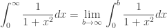
The value is the same. While that is pretty straightforward, there are other things going on here which may be enlightening. The original indefinite integral represents the area in the first quadrant between the graph of $y=\frac{1}{1+{{x}^{2}}}$ and the x-axis. Let’s consider the function that gives the area between the y-axis and the vertical line at various values of x.

$A \displaystyle\left( x \right)=\int_{0}^{x}{\frac{1}{1+{{t}^{2}}}}\ dt$

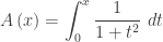
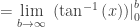
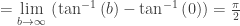
Pretending for the moment that we don’t know the antiderivative, we can use a calculator to graph the area function. Of course, we recognize this as the inverse tangent function, but what is more interesting is that whatever this function is, it seems to have a horizontal asymptote at $y=\tfrac{\pi }{2}$ . The area is approaching a finite limit as x increases without bound. The unbounded region has a finite area. The connection with improper integrals is obvious.

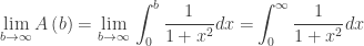
$\displaystyle \underset{b\to \infty }{\mathop{\lim }}\,A\left( b \right)=\underset{b\to \infty }{\mathop{\lim }}\,\int_{0}^{b}{\frac{1}{1+{{x}^{2}}}dx=}\int_{0}^{\infty }{\frac{1}{1+{{x}^{2}}}dx}$

Also, the improper integral is defined as the limit of the area function. This may give some insight as to why improper integrals are defined as they are.

Modified Tabular Integration

Posted on July 24, 2013 by Lin McMullin

Several weeks ago, Dr. Qibo Jing, an AP teacher at Rancho Solano Preparatory School in Scottsdale, Arizona, posted a new way to approach tabular integration to the AP Calculus Community discussion group. He calls this the Modified Tabular Method. The algorithm makes repeated integration by parts quicker and more streamlined than the usual method. The usual method is explained here.

Here is Dr. Jing’s method outlined and illustrated with this example $\displaystyle I=\int{\left( {{x}^{3}}+7{{x}^{2}} \right)\cos \left( x \right)dx}$

Step 1: Identify u and dv in the usual way and rewrite the given integral in terms of $u={{x}^{3}}+7{{x}^{2}}$ and $dv=\cos \left( x \right)=\tfrac{d}{dx}\sin \left( x \right)$ .

$\displaystyle I=\int{\left( {{x}^{3}}+7{{x}^{2}} \right)\cos \left( x \right)dx}=\int{\left( {{x}^{3}}+7{{x}^{2}} \right)\left( \tfrac{d}{dx}\left( \sin x \right) \right)}$

Step 2: The first term of the antiderivative is the product of the two functions that appear in the revised integral:

$\displaystyle I=\int{\left( {{x}^{3}}+7{{x}^{2}} \right)\left( \tfrac{d}{dx}\left( \sin x \right) \right)}=\left( {{x}^{3}}+7{{x}^{2}} \right)\sin \left( x \right)\cdots$

Step 3: The remaining terms alternate sign. The next term has subtraction sign etc. The first factor of the next term is the derivative of the first factor of the current term. The second factor is the antiderivative of the second factor of the current term – differentiate the first factor; integrate the second factor.

$\displaystyle I =\int{\left( {{x}^{3}}+7{{x}^{2}} \right)\left( \tfrac{d}{dx}\left( \sin x \right) \right)}=\left( {{x}^{3}}+7{{x}^{2}} \right)\sin \left( x \right)-\left( 3{{x}^{2}}+14x \right)\left( -\cos \left( x \right) \right)\cdots$

Step 4: Alternate signs and repeat step 3 until the term becomes zero or until the original form appears (See next example). DO NOT simplify either factor until you are done as this may change later terms.

The simplified result is

$\displaystyle I=\left( {{x}^{3}}+7{{x}^{2}}-6x-14 \right)\sin \left( x \right)+\left( 3{{x}^{2}}+14x-6 \right)\cos \left( x \right)+C$

Here is a second example. In this example the original integral returns as the third term.

$\displaystyle I=\int{{{e}^{x}}\sin \left( x \right)dx=\int{\sin \left( x \right)\left( \tfrac{d}{dx}{{e}^{x}}dx \right)}}$

$=\sin \left( x \right)\left( {{e}^{x}} \right)-\cos \left( x \right)\left( {{e}^{x}} \right)+\left( -\sin \left( x \right) \right)\left( {{e}^{x}} \right)$

$={{e}^{x}}\sin \left( x \right)-\cos \left( x \right)\left( {{e}^{x}} \right)-I$

$2I={{e}^{x}}\sin \left( x \right)-\cos \left( x \right)\left( {{e}^{x}} \right)$

$I=\tfrac{1}{2}\left( {{e}^{x}}\sin \left( x \right)-\cos \left( x \right)\left( {{e}^{x}} \right) \right)+C$

This really is a simpler algorithm than the usual tabular method.

Variations on a Theme by ETS

Posted on June 14, 2013 by Lin McMullin

Experienced AP calculus teacher use as many released exam questions during the year as they can. They are good questions and using them gets the students used to the AP style and format. They can be used “as is”, but many are so rich that they can be tweaked to test other concepts and to make the students think wider and deeper.

Below is a multiple-choice question from the 2008 AB calculus exam, question 9.

The graph of the piecewise linear function f is shown in the figure above. If $\displaystyle g\left( x \right)=\int_{-2}^{x}{f\left( t \right)\,dt}$ , which of the following values is the greatest?

(A) g(-3) (B) g(-2) (C) g(0) (D) g(1) (E) g(2)

I am now going to suggest some ways to tweak this question to bring out other ideas. Here are my suggestions. Some could be multiple-choice others simple short constructed response questions. A few of these questions, such as 3 and 4, ask the same thing in different ways.

1. 1. Require students to show work or justify their answer even on multiple-choice questions. So for this question they should write, “The answer is (D) g(1) since x = 1 is the only place where ${g}'\left( x \right)=f\left( x \right)$ changes from positive to negative.”
  2. Ask, “Which of the following values is the least?” (Same choices)
  3. Find the five values listed.
  4. Put the five values in order from smallest to largest.
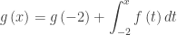
  5. If $\displaystyle g\left( x \right)=g\left( -2 \right)+\int_{-2}^{x}{f\left( t \right)dt}$ and the maximum value of g is 7, what is the minimum value?
  6. If $\displaystyle g\left( x \right)=g\left( -2 \right)+\int_{-2}^{x}{f\left( t \right)dt}$ and the minimum value of g is 7, what is the maximum value?
  7. Pick any number (not just an integers) in the interval [–3, 2] to be a and change the stem to read, “If $\displaystyle g\left( x \right)=g\left( a \right)+\int_{a}^{x}{f\left( t \right)dt}$ ….” And then ask any of the questions above – some answers will be different, some will be the same. Discussing which will not change and why makes a worthwhile discussion.
  8. Change the equation in the stem to $\displaystyle g\left( x \right)=3x+\int_{-2}^{x}{f\left( t \right)dt}$ and ask the questions above. Again most of the answers will change. Also this question and the next start looking like some free-response questions. Compare them with 2011 AB 4 and 2010 AB 5(c)
  9. Change the equation in the stem to $\displaystyle g\left( x \right)=-\tfrac{3}{2}x+\int_{-2}^{x}{f\left( t \right)dt}$ and ask the questions above. This time most of the answers will change.
  10. Change the graph and ask the same questions.

Not all questions offer as many variations as this one. For some about all you can do is use them “as is” or just change the numbers.

Any other adaptations you can think of?

What is your favorite question for tweaking?

Math in the News Combinatorics and UPS

Revised: August 24, 2014

Why You Never Need Cylindrical Shells

Posted on January 14, 2013 by Lin McMullin

Don’t get me wrong; finding volumes of solids of rotation by the method of cylindrical shells is a great method. It’s just that you can always work around it; you don’t ever need to use it. The work-around is often longer and involves more work, but it is interesting mathematically. So here’s an example of how to do it.

The region bounded by the graph of $y={{x}^{3}}+x+1$ , and the lines y = 1 and x = 2, is revolved around the y-axis. What is the volume of the resulting solid?

Supposedly this volume must be found by the shell method. Using the washer method the volume is set up as the integral of the area of the outside circle with constant radius of 2, minus the area of the inside circle of radius x, times the “thickness” of a slice. This “thickness” is in the y-direction and so is dy. The dy also determines the limits of integration.

$\displaystyle V=\int_{1}^{11}{\left( \pi {{2}^{2}}-\pi {{x}^{2}} \right)\,dy}$

Since the integral contains a dy the usual way is to change the x to a function of y, which in this case involves solving a cubic polynomial. In this case that is very difficult to find x as a function of y and with a different function that may even be impossible. But do we really have to do that? In fact, what is required is to have only one variable and the variable may be x! So we find dy in terms of x and dx and substitute into the expression above. We also change the limits of integration to the corresponding x-values.

$dy=\left( 3{{x}^{2}}+1 \right)dx$
$\displaystyle V=\int_{0}^{2}{\left( \pi {{2}^{2}}-\pi {{x}^{2}} \right)\,\left( 3{{x}^{2}}+1 \right)dx}$
$\displaystyle V=\pi \int_{0}^{2}{\left( 4+11{{x}^{2}}-3{{x}^{4}}\, \right)dx}$

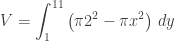
This integral is easy to evaluate and will give the same value, $\tfrac{272}{15}\pi$ , as the shell integral.

To use this idea, the function must either be one-to-one on the interval or the solid must be broken into sections that are one-to-one. This may make the problem longer. Most problems that you want to do by shells are easier by shells. The point is that washers (or disks) may always be used; not that the washer approach is the easiest way.

Jobs, Jobs, Jobs

Posted on December 5, 2012 by Lin McMullin

Here is a problem similar to those in the last two posts; this one is based on a graph. The numbers are a little hard to read (sorry), but perhaps we do not need them. (If you want to do the numbers it is the second graph from the source which is more readable. There are other graphs of this type in the source, if you want some more.)

The discussion is aimed at relating the graph which is a derivative with the net change it describes. Thus, we are looking at determining increasing, decreasing, and relative extreme value from the graph and foreshadowing how this can be done using integration concepts especially accumulation.

Source: The Bureau of Labor Statistics

Some questions to discuss.

1. What are the units of this data, and what kind of units are they? (Thousands of jobs per month – a rate unit.)
2. Ask the students how they would find the total change in employment over the period given and discuss this with them. (Do not make them do the computation, just discuss how.)
3. Ask them to indicate on the graph when the total employment was the least and explain how they can tell from the graph (January 2010 – this is where the rate changes from negative to positive; this is the graph of a rate in thousands of jobs per month, therefore it is the derivative of jobs (employment)).
4. Ask how they could verify this by computing. What would they compute month-by-month? (The total number of jobs lost or gained from the beginning of the period – the accumulated change in jobs.)
5. During 2010 there is a local maximum in employment and another (local) minimum: when do they occur? How do you know without doing a computation?
6. What additional information do you need to tell how many people actually had jobs at any time during this period? (The total number employed at the beginning of 2008 – the initial condition.)

Teaching Calculus

The pleasure lies not in discovering the truth, but in searching for it.

Tag Archives: Integration

Graphing Integrals