Unit 9 includes all the topics listed in the title. These are BC only topics (CED – 2019 p. 163 – 176). These topics account for about 11 – 12% of questions on the BC exam.
Comments on Prerequisites: In BC Calculus the work with parametric, vector, and polar equations is somewhat limited. I always hoped that students had studied these topics in detail in their precalculus classes and had more precalculus knowledge and experience with them than is required for the BC exam. This will help them in calculus, so see that they are included in your precalculus classes.
Topics 9.1 – 9.3 Parametric Equations
Topic 9.1: Defining and Differentiation Parametric Equations. Finding dy/dx in terms of dy/dt and dx/dt
Topic 9.3: Finding Arc Lengths of Curves Given by Parametric Equations.
Topics 9.4 – 9.6 Vector-Valued Functions and Motion in the plane
Topic 9.4 :Defining and Differentiating Vector-Valued Functions. Finding the second derivative. See this A Vector’s Derivatives which includes a note on second derivatives.
Topic 9.5: Integrating Vector-Valued Functions
Topic 9.6: Solving Motion Problems Using Parametric and Vector-Valued Functions. Position, Velocity, acceleration, speed, total distance traveled, and displacement extended to motion in the plane.
Topics 9.7 – 9.9 Polar Equation and Area in Polar Form.
Topic 9.7: Defining Polar Coordinate and Differentiation in Polar Form. The derivatives and their meaning.
Topic 9.8: Find the Area of a Polar Region or the Area Bounded by a Single Polar Curve
Topic 9.9: Finding the Area of the Region Bounded by Two Polar Curves. Students should know how to find the intersections of polar curves to use for the limits of integration.
Timing
The suggested time for Unit 9 is about 10 – 11 BC classes of 40 – 50-minutes, this includes time for testing etc.
A recent post on the AP Calculus bulletin board observed that the maximum value of the average value of a function on an interval occurred at the point where the graph of the average value and the function intersect. I am not sure if this concept is important in and of itself, but it does make an interesting exercise.
For a function f(x), we may treat its average value as a function, A(x), defined for all x ∈ [a, b], interval [a, x] as
Graphically, the segment drawn at y = A(x) is such that the regions between the line and the function above and below the segment have equal areas. See figure 1 in which the red curve is the function, and the blue curve is the average value function. The two shaded regions have the same area.
Figure 1: The shaded regions have the same area.
Regardless of the starting value, the function and its average value start at the same value. If the function is increasing the average value is less than the function and increasing. When the function starts to decrease, the average value will continue to increase for a while. When the two graphs nest intersect, the process starts over, and the average value will now start to decrease. Therefore, the intersection value is when the average value function change from increasing to decreasing and this is its (local) maximum value. See Figure 2.
Figure 2:The maximum value of A(x) is at the intersection of the two graphs
This continues until the graphs intersect again after the function starts to increase: a (local) minimum value of the average value function. The process continues with the extreme values of the average value function (blue graph) occurring at its intersections with the function. Figure 3
Figure 3: A(x) has its extreme values where it intersects the function.
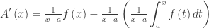
This can be proved by finding the extreme values of the average value function by considering its derivative. Begin by finding its derivative using the product rule (or quotient rule) and the FTC.
The critical points of a(x) occur when its derivative is equal to zero (or undefined). This is when (or when x = a, the endpoint). This is where the graphs intersect.
How to use this in your class
This is not a concept that is likely to be tested on the AP Calculus Exams. Nevertheless, it is an easy enough idea to explore when teaching the average value of a function and at the same time reviewing some earlier concepts such as product (or quotient) rule, the FTC (differentiating an integral), and some non-ordinary simplification.
You could have your students use their own favorite function and show that the extreme values of its average value occur where the average value intersects the function. This is good practice in equation solving on a calculator since the points do not occur at “nice” numbers. Here’s an example.
If , then its average value on the interval is
.
The intersections of f(x) and A(x) can be found by solving
The extreme values of may also be found using a calculator.
The points are the same. the first is approximately (2.331, 0.725) and the second is (6.283, 0) or (2π, 0). This second is reasonable since at 2π the sine function has completed one period and its average value zero. (See figure 3 again.).
Other questions you could ask (for my function anyway) are what is the absolute maximum and how can you be sure? Why are all the minimums zero?
The message on the AP Calculus discussion boards that inspired this post was started by Neema Salimi an AP Calculus teacher from Georgia. He made the original observation. You can read his original post and proof, and comments by others here.
The Rule of Four
Not much has been heard of the Rule of Four lately. The Rule of Four suggests that mathematical concepts should be looked at graphically, numerically, analytically, and verbally. It has not gone away. The Rule of Four has a new name: multiple representations. (In the latest Course and Exam Description, you will find it in Mathematical Practices (p. 14), specifically practices 2.B, 2.C, 2.D, 2.E, 3.E, 3.F, 4.A, and 4.C)
I have used the Rule of Four in this post. The post started with a verbal discussion of the concept and how the result can be seen graphically. That was followed by analytic proof. At the end is a numerical example.
Other posts on the average value of a function:
Finding the average value of a function on an interval is Topic 8.1 in the Course and Exam Description (p. 149)
What’s a Mean Old Average Anyway? Be sure to distinguish between the average rate of change, the average value of a function, and the mean value theorem.
I’ve never liked memorizing formulas. I would rather know where they came from or be able to tie it to something I already know. One of my least favorite formulas to remember and explain was the formula for the second derivative of a curve given in parametric form. No longer.
If and, then the traditional formulas give
, and
It is that last part, where you divide by , that bothers me. Where did the come from?
Then it occurred to me that dividing by is the same as multiplying by
It’s just implicit differentiation!
Since is a function of t you must begin by differentiating the first derivative with respect to t. Then treating this as a typical Chain Rule situation and multiplying by gives the second derivative. (There is a technical requirement here that given , then its inverse exists.)
In fact, if you look at a proof of the formula for the first derivative, that’s what happens there as well:
The reason you do it this way is that since x is given as a function of t, it may be difficult to solve for t so you can find dt/dx in terms of x. But you don’t have to; just divide by dx/dt which you already know.
Here is an example for both derivatives.
Suppose that and
Then and and
Then
And
Yes, it’s the same thing as using the traditional formula, but now I’ll never have to worry about forgetting the formula or being unsure how to explain why you do it this way.
Revised: Correction to last equation 5/18/2014. Revised: 2/8/2016. Originally posted May 5, 2014.
About this time of year, you find someone, hopefully one of your students, asking, “If I’m finding where a function is increasing, is the interval open or closed?”
Do you have an answer?
This is a good time to teach some things about definitions and theorems.
The place to start is to ask what it means for a function to be increasing. Here is the definition:
A function is increasing on an interval if, and only if, for all (any, every) pairs of numbers x1 < x2 in the interval, f(x1) < f(x2).”
(For decreasing on an interval, the second inequality changes to f(x1) > f(x2). All of what follows applies to decreasing with obvious changes in the wording.)
Notice that functions increase or decrease on intervals, not at individual points. We will come back to this in a minute.
Numerically, this means that for every possible pair of points, the one with the larger x-value always produces a larger function value.
Graphically, this means that as you move to the right along the graph, the graph is going up.
Analytically, this means that we can prove the inequality in the definition.
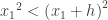
For an example of this last point consider the function f(x) = x2. Let x2 = x1 + h where h > 0. Then in order for f(x1) < f(x2) it must be true that
This can only be true if Thus, x2 is increasing only if
Now, of course, we rarely, if ever, go to all that trouble. And it is even more trouble for a function that increases on several intervals. The usual way of finding where a function is increasing is to look at its derivative.
Notice that the expression looks a lot like the numerator of the original limit definition of the derivative of x2 at x = x1, namely . If h > 0, where the function is increasing the numerator is positive and the derivative is positive also. Turning this around we have a theorem that says, If for all x in an interval, then the function is increasing on the interval. That makes it much easier to find where a function is increasing, we simplify find where its derivative is positive.
There is only a slight problem in that the theorem does not say what happens if the derivative is zero somewhere on the interval. If that is the case, we must go back to the definition of increasing on an interval or use a different method. For example, the function x3 is increasing everywhere, even though its derivative at the origin is zero.
Let’s consider another example. The function sin(x) is increasing on the interval (among others) and decreasing on . It bothers some that is in both intervals and that the derivative of the function is zero at x = . This is not a problem. Sin() is larger than all the other values is both intervals, so by the definition, and not the theorem, the intervals are correct.
It is generally true that if a function is continuous on the closed interval [a,b] and increasing on the open interval (a,b) then it must be increasing on the closed interval [a,b] as well.
Returning to the first point above: functions increase or decrease on intervals not at points. You do find questions in books and on tests that ask, “Is the function increasing at x = a.” The best answer is to humor them and answer depending on the value of the derivative at that point. Since the derivative is a limit as h approaches zero, the function must be defined on some interval around x = a in which h is approaching zero. So, answer according to the value of the derivative on that interval.
Every function that is continuous on a closed interval must have a maximum and a minimum value on the interval. These values may all be the same (y = 2 on [-3,3]); or the function may reach these values more than once (y = sin(x)).
If the function is defined on a closed interval, then the extreme values are either (1) at an endpoint of the interval or (2) at a critical number. This is known as the Extreme Value Theorem. Thus, one way of finding the extreme values is to simply find the value of the function at the endpoints and the critical points and compare these to find the largest and smallest. This is called the Candidates’ Test or the Closed Interval Test. It is a good one to “play” with: do some sketches of the different situation above; discuss why the interval must be closed.
On an open or closed interval, the shapes can change if the first derivative is zero or undefined at the point where two shapes join. In this case the point is a local extreme value of the function – a local maximum or minimum value. Specifically:
If the first derivative changes from positive to negative, the shape of the function changes from increasing to decreasing and the point is a local maximum. If the first derivative changes from negative to positive, the shape of the function changes from decreasing to increasing and the point is a local minimum.
This is a theorem called the First Derivative Test. By finding where the first derivative changes sign and in which direction it changes (positive to negative, or negative to positive) we can locate and identify the local extreme value precisely.
Another way to determine if a critical number is the location of a local maximum or minimum is a theorem called the Second Derivative Test.
If the first derivative is zero (and specifically not if it is undefined) and the second derivative is positive, then the graph has a horizontal tangent line and is concave up. Therefore, this is the location of a local minimum of the function.
Likewise, if the first derivative is zero at a point and the second derivative is negative there, the function has a local maximum there.
If both the first and second derivatives are zero at a point, then the second derivative test cannot be used, for example y = x4 at the origin.
The mistake students make with the second derivative test is in not checking that the first derivative is zero. If “justify your answer” is required, students should be sure to show that the first derivative is zero as well as the sign of the second derivative.
In the case where both the first and second derivatives are zero at the same point the function changes direction but not concavity (e.g. f (x) = x4 at the origin), or changes concavity but not direction (e.g. f (x) = x3 at the origin).
This is a revised version of a post published on October 22, 2012
A very typical calculus problem is given the equation of a function, to find information about it (extreme values, concavity, increasing, decreasing, etc., etc.). This is usually done by computing and analyzing the first derivative and the second derivative. All the textbooks show how to do this with copious examples and exercises. I have nothing to add to that. One of the “tools” of this approach is to draw a number line and mark the information about the function and the derivative on it.
A very typical AP Calculus exam problem is given the graph of the derivative of a function, but not the equation of either the derivative or the function, to find all the same information about the function. For some reason, students find this difficult even though the two-dimensional graph of the derivative gives all the same information as the number line graph and, in fact, a lot more.
Looking at the graph of the derivative in the x,y-plane it is easy to determine the important information. Here is a summary relating the features of the graph of the derivative with the graph of the function.
Feature
the function
> 0
is increasing
< 0
is decreasing
changes – to +
has a local minimum
changes + to –
has a local maximum
increasing
is concave up
decreasing
is concave down
extreme value
has a point of inflection
Here’s a typical graph of a derivative with the first derivative features marked.
Here is the same graph with the second derivative features marked.
The AP Calculus Exams also ask students to “Justify Your Answer.” The table above, with the columns switched does that. The justifications must be related to the given derivative, so a typical justification might read, “The function has a relative maximum at x = -2 because its derivative changes from positive to negative at x = -2.”
The Mean Value Theorem (MVT) is proved by writing the equation of a function giving the (directed) length of a segment from the given function to the line between the endpoints as you can see here. Since the function and the line intersect at the endpoints of the interval this function satisfies the hypotheses of Rolle’s theorem and so the MVT follows directly. This means that the derivative of the distance function is zero at the points guaranteed by the MVT. Therefore, these values must also be the location of the local extreme values (maximums and minimums) of the distance function on the open interval. *
Here is an exploration in three similar examples that use this idea to foreshadow the MVT. You, of course, can use your own favorite function. Any differentiable function may be used, in which case a CAS calculator may be helpful. Answers are at the end.
First example:
Consider the function defined on the closed interval [–1,3]
Write the equation of the line thru the endpoints of the function.
Write an expression for h(x) the vertical distance between f(x) and the line found in part 1.
Find the x-coordinates of the local extreme values of h(x) on the open interval (–1,3).
Find the slope of f(x) at the values found in part 3.
Compare your answer to part 4 with the slope of the line. Is this a coincidence?
Second example: slightly more difficult than the first.
Consider the function defined on the closed interval .
Write the equation of the line thru the endpoints of the function.
Write an expression for h(x) the vertical distance between f(x) and the line found in part 1.
Find the x-coordinates of the local extreme values of h(x) on the open interval .
Find the slope of f(x) at the values found in part 3.
Compare your answer to part 4 with the slope of the line. Is this a coincidence?
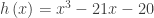
Third example: In case you think I cooked the numbers. You may want to use a CAS for this one.
Consider the function defined on the closed interval .
Write the equation of the line thru the endpoints of the function.
Write an expression for h(x) the vertical distance between f(x) and the line found in part 1.
Find the x-coordinates of the local extreme values of h(x) on the open interval .
Find the slope of f(x) at the values found in part 3.
Compare your answer to part 4 with the slope of the line. Is this a coincidence?
Answers
First example:
y = x
when x = –1/2, ½, 3/2 and 5/2
, the slope = 1 at all four points
They are the same. Not a coincidence.
Second example:
The endpoints are and ; the line is
when
; at the points above the slope is 1.
They are the same. Not a coincidence.
Third example:
The endpoints are (-4, -64) and (5, 125), the line is .
when
They are the same. Not a coincidence.
See this post for links to other posts discussing the full development of the MVT
* It is possible that the derivative is zero and the point is not an extreme value. This is like the situation with a point of inflection when the first derivative is zero but does not change sign.
This post was originally published on October 19, 2018.


 (or when x = a, the endpoint). This is where the graphs intersect.
 , then its average value on the interval
  is
is  .
. 
 may also be found using a calculator.
  and,
and,  then the traditional formulas give
 , and
, and
 , that bothers me. Where did the
 is a function of t you must begin by differentiating the first derivative with respect to t. Then treating this as a typical Chain Rule situation and multiplying by
  exists.)
 and
and 
 and
and  and
and 


 Thus, x2 is increasing only if
 for all x in an interval, then the function is increasing on the interval. That makes it much easier to find where a function is increasing, we simplify find where its derivative is positive.
![\displaystyle [-\tfrac{\pi }{2},\tfrac{\pi }{2}]](https://s0.wp.com/latex.php?latex=%5Cdisplaystyle+%5B-%5Ctfrac%7B%5Cpi+%7D%7B2%7D%2C%5Ctfrac%7B%5Cpi+%7D%7B2%7D%5D&bg=ffffff&fg=333333&s=0&c=20201002) (among others) and decreasing on
(among others) and decreasing on ![\displaystyle [\tfrac{\pi }{2},\tfrac{3\pi }{2}]](https://s0.wp.com/latex.php?latex=%5Cdisplaystyle+%5B%5Ctfrac%7B%5Cpi+%7D%7B2%7D%2C%5Ctfrac%7B3%5Cpi+%7D%7B2%7D%5D&bg=ffffff&fg=333333&s=0&c=20201002) . It bothers some that
. It bothers some that  is in both intervals and that the derivative of the function is zero at x =
  > 0
> 0

 defined on the closed interval [–1,3]
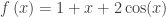 defined on the closed interval
 ![\displaystyle [\tfrac{\pi }{2},\tfrac{{9\pi }}{2}]](https://s0.wp.com/latex.php?latex=%5Cdisplaystyle+%5B%5Ctfrac%7B%5Cpi+%7D%7B2%7D%2C%5Ctfrac%7B%7B9%5Cpi+%7D%7D%7B2%7D%5D&bg=ffffff&fg=333333&s=0&c=20201002) .
. .
. defined on the closed interval
 ![\displaystyle [-4,5]](https://s0.wp.com/latex.php?latex=%5Cdisplaystyle+%5B-4%2C5%5D&bg=ffffff&fg=333333&s=0&c=20201002) .
. .
.
 when x = –1/2, ½, 3/2 and 5/2
 , the slope = 1 at all four points
 and
and  ; the line is

 when
when 
 ; at the points above the slope is 1.
 .
.
 when
when 

