Variations on a Theme by ETS

Experienced AP calculus teacher use as many released exam questions during the year as they can. They are good questions and using them gets the students used to the AP style and format.  They can be used “as is”, but many are so rich that they can be tweaked to test other concepts and to make the students think wider and deeper.  

Below is a multiple-choice question from the 2008 AB calculus exam, question 9.

 2008 mc9The graph of the piecewise linear function f  is shown in the figure above. If \displaystyle g\left( x \right)=\int_{-2}^{x}{f\left( t \right)\,dt}, which of the following values is the greatest?

(A)  g(-3)         (B)  g(-2)         (C)  g(0)         (D)  g(1)         (E)  g(2)

I am now going to suggest some ways to tweak this question to bring out other ideas. Here are my suggestions. Some could be multiple-choice others simple short constructed response questions. A few of these questions, such as 3 and 4, ask the same thing in different ways.

      1. Require students to show work or justify their answer even on multiple-choice questions. So for this question they should write, “The answer is (D) g(1) since x = 1 is the only place where {g}'\left( x \right)=f\left( x \right) changes from positive to negative.” 
      2. Ask, “Which of the following values is the least?” (Same choices)
      3. Find the five values listed.
      4. Put the five values in order from smallest to largest.
      5. If \displaystyle g\left( x \right)=g\left( -2 \right)+\int_{-2}^{x}{f\left( t \right)dt} and the maximum value of g is 7, what is the minimum value?
      6. If \displaystyle g\left( x \right)=g\left( -2 \right)+\int_{-2}^{x}{f\left( t \right)dt} and the minimum value of g is 7, what is the maximum value?
      7. Pick any number (not just an integers) in the interval [–3, 2] to be a and change the stem to read, “If \displaystyle g\left( x \right)=g\left( a \right)+\int_{a}^{x}{f\left( t \right)dt} ….” And then ask any of the questions above – some answers will be different, some will be the same. Discussing which will not change and why makes a worthwhile discussion.
      8. Change the equation in the stem to \displaystyle g\left( x \right)=3x+\int_{-2}^{x}{f\left( t \right)dt} and ask the questions above. Again most of the answers will change. Also this question and the next start looking like some free-response questions. Compare them with 2011 AB 4 and 2010 AB 5(c)
      9. Change the equation in the stem to \displaystyle g\left( x \right)=-\tfrac{3}{2}x+\int_{-2}^{x}{f\left( t \right)dt} and ask the questions above. This time most of the answers will change.
      10. Change the graph and ask the same questions.

Not all questions offer as many variations as this one. For some about all you can do is use them “as is” or just change the numbers.

Any other adaptations you can think of?

What is your favorite question for tweaking?

 Math in the News Combinatorics and UPS

Revised: August 24, 2014

L’Hôpital Rules the Graph

In my last post on May 31, 2012 I showed a way of demonstrating why L’Hôpital’s Rule works. We looked at an example,

\displaystyle \underset{x\to \pi }{\mathop{\lim }}\,\frac{\tan \left( x \right)}{\sin \left( x \right)},

which met the requirement of the theorem called L’Hôpital’s Rule, namely the functions are differentiable and, since  tan(\pi ) = sin(\pi ) = 0 they intersect on the x-axis at \left( \pi ,0 \right)
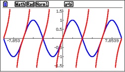
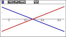
. We looked at the graph and then zoomed-in at
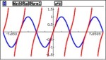
 \left( \pi ,0 \right).

L’Hôpital’s Rule tells us that with these conditions the limit is the same as the limit of the ratio of their slopes (or their derivatives, if you prefer). Can you see what that ratio is from Figure 2? Even though this is not a “square window” the ratio is obviously –1.

Here are four other limits. See if you can find them by the method suggested here. Namely zoom-in on the point where the functions intersect and see if you can find the limits without doing any computations. (Yes, I know you already know the first 3, but try this idea anyway. )

1. \displaystyle \underset{x\to 0}{\mathop{\lim }}\,\frac{\sin \left( x \right)}{x}

2. \displaystyle \underset{x\to 0}{\mathop{\lim }}\,\frac{1-\cos \left( x \right)}{x}

3. \displaystyle \underset{x\to 0}{\mathop{\lim }}\,\frac{\cos \left( \tfrac{\pi }{2}+x \right)}{x} also known as \displaystyle \underset{x\to 0}{\mathop{\lim }}\,\frac{\cos \left( \tfrac{\pi }{2}+x \right)-\cos \left( \tfrac{\pi }{2} \right)}{x}

4. \displaystyle \underset{x\to 1}{\mathop{\lim }}\,\frac{\pi \ln \left( x \right)}{\sin \left( \pi x \right)}


Answers in order:  1, 0, -1, -1

Locally Linear L’Hôpital

I’ll begin with a lemma. (I like to do a lemma now and then if for no other reason than having an excuse to explain what a lemma is – a simple theorem that is used in proving the main theorem.)

Lemma: If two lines intersect on the x-axis, then for any x the ratio of their y-coordinates is equal to the ratio of their slopes.

Proof: Two lines with slopes of m1 and m2 that intersect at (a, 0) on the x-axis have equations y1 = m1(xa) and y2 = m2(xa). Then

\displaystyle \frac{{{y}_{1}}}{{{y}_{2}}}=\frac{{{m}_{1}}\left( x-a \right)}{{{m}_{2}}\left( x-a \right)}=\frac{{{m}_{1}}}{{{m}_{2}}}

L’Hôpital’s Rule (Theorem): If f and g are differentiable near x = a and f(a) = g(a) = 0, then

\displaystyle \underset{x\to a}{\mathop{\lim }}\,\frac{f\left( x \right)}{g\left( x \right)}=\underset{x\to a}{\mathop{\lim }}\,\frac{{f}'\left( x \right)}{{g}'\left( x \right)}

if the limit exists.

The fact that f(a) = g(a) = 0 means that the two functions intersect on the x-axis at (a, 0). For example, the functions f(x) = tan(x) and g(x) = sin(x) have this property at \left( \pi ,0 \right).

Figure 1. y = tan(x) in red and y = sin(x) in blue

Figure 1. y = tan(x) in red and y = sin(x) in blue

Now zoom-in several times centered at \left( \pi ,0 \right).

Figure 2. The previous graph zoomed in.

Figure 2. The previous graph zoomed in.

Whoa!

That looks like lines!!

It’s the local linearity property of differentiable functions – if you zoom-in enough any differentiable function eventually looks linear. So maybe near \left( \pi ,0 \right) the lemma applies. The only difference is that the slopes of the “lines” are the derivatives so

\displaystyle \underset{x\to a}{\mathop{\lim }}\,\frac{f\left( x \right)}{g\left( x \right)}=\underset{x\to a}{\mathop{\lim }}\,\frac{{f}'\left( x \right)}{{g}'\left( x \right)}

 Now that does not quite prove L’Hôpital’s Rule, but it should give you and your students a good idea of why L’Hôpital’s Rule is true.

Then in our example:

\displaystyle \underset{x\to \pi }{\mathop{\lim }}\,\frac{\tan \left( x \right)}{\sin \left( x \right)}=\underset{x\to \pi }{\mathop{\lim }}\,\frac{\frac{1}{{{\left( \cos \left( x \right) \right)}^{2}}}}{\cos \left( x \right)}=\underset{x\to \pi }{\mathop{\lim }}\,\frac{1}{{{\left( \cos \left( x \right) \right)}^{3}}}=\frac{1}{{{\left( \cos \left( \pi \right) \right)}^{3}}}=-1

But isn’t that obvious from Figure 2?

Think about it.

More on this next time.


A Standard Problem?

Sometimes even the simplest problems can lead to interesting places. I got interested in this ordinary textbook problem a few months ago while observing an AB calculus class. Here is how my thinking went written as a series of exercises:

Original exercise: Find the point(s) on the parabola y = x2 that are closest to the point (0, 2).

The solution is straightforward:

Let z(x) be the distance from (0, 2) to the point (x, x2). Then \displaystyle z\left( x \right)=\sqrt{{{\left( x-0 \right)}^{2}}+{{\left( {{x}^{2}}-2 \right)}^{2}}}and setting the derivative equal to zero, we find the critical points at x = 0 a local maximum and x=-\sqrt{\tfrac{3}{2}} and x=\sqrt{\tfrac{3}{2}} both absolute minimums located symmetrically to the y-axis.

The students had some trouble understanding what was going on. I suggested they consider a point moving along the parabola starting high on the left side. As the point comes down the graph its distance from \left( 0,2 \right) gets shorter until it reaches some minimum length somewhere. Then the distance gets longer again until – where? Obviously, at the origin. Then symmetry takes over and the distance decreases again until it reaches a second minimum directly across the y-axis from the first point, after which it increases forever.

Exercise 1: Sketch the graph of the distance function, z(x), on top of the graph of the parabola. Give the exact coordinates of the maximum point without doing any computations. Discuss the y-coordinates of the minimum points.

It then occurred to me that there is nothing sacred about (0, 2). We could use any point on the y-axis, . Or could we? I pictured a circle centered at the point (0, a) on the y-axis tangent to the parabola (i.e. tangent to the tangent line of the parabola). The radius of such a circle is the minimum distance for that y-axis center point.

Exercise 2: If the point is below the origin then obviously the minimum distance is the distance directly up to the origin. There are places above the x-axis where the origin is the closest point. For what values of a is the origin the closest point? Use the circle mentioned above to explain how this is possible.

The distance graph that we drew above has a W shape similar to the shape of some 4th degree polynomials (note: z(x) is not a 4th degree polynomial, it is not even a polynomial). So next I drew the graph of z’(x), the first derivative of z; this graph is similar to a cubic polynomial (again it is not a polynomial)

Exercise 3: Without actually computing the derivative’s equation, sketch the graph of the derivative with the graph of the parabola and the distance function’s graph. Be sure the critical points are where they should be.

Exercise 4: Use a graphing program or a graphing calculator do draw the parabola, z(x) and z’(x) and use it to check your sketches.

Project: Using a suitable program (Winplot, Geogebra, etc.) set up an animation that will show all the features discussed above. It should show the parabola which does not move, the movable point (0, a), the circle tangent to the parabola, z(x) and z’(x). These last 3 should move with the slider for a.

At this point I noticed that the derivative changed concavity 4 times (up-down-up-down). The origin is one of 3 points of inflection. I wondered if there was anything interesting about the location of the points of inflection.

Exercise 5: Find the coordinates of the points of inflection of z’(x). Are they related to any of the features in the problem? (Use a CAS for this one.)

The solutions can be found here: Closest Point Problem Solution.

What’s a Mean Old Average Anyway?

Students often confuse the several concepts that have the word “average” or “mean” in their title. This may be partly because not just the names, but the formulas associated with each are very similar, but I think the main reason may be that they are keying in on the word “average” rather than the full name.

Here are the three items. We will assume that the function f is continuous on the closed interval [a, b] and differentiable on the open interval (a, b):

1.  The average rate of change of a function over the interval is simply the slope of the line from one endpoint of the graph to the other.

 \displaystyle \frac{f\left( b \right)-f\left( a \right)}{b-a}

2. The mean (or average) value theorem say that somewhere in the open interval (a, b) there is a number c such that the derivative (slope) at x = c is equal to the average rate of change over the interval.

\displaystyle {f}'\left( c \right)=\frac{f\left( b \right)-f\left( a \right)}{b-a}

3. The average value of a function is literally the average of all the y-coordinates on the interval. It is the vertical side of a rectangle whose base extends on the x-axis from x = a to x =b and whose area is the same as the area between the graph and the x-axis and the function over the same interval.

\displaystyle \frac{\int_{a}^{b}{f\left( x \right)dx}}{b-a}

Notice that when you evaluate the integral, the result looks very much like the ones above. This formula is also called the mean value theorem for integrals or the integral form of the mean value theorem. No wonder people get confused.

The three are closely related. Consider a position-velocity-acceleration situation. The average rate of change of position (#1 above) is the average value of the velocity (#3) and somewhere the velocity must equal this number (#2). Similarly, the average rate of change of velocity (#1) is the average acceleration (#3) and somewhere in the interval the acceleration (derivative of velocity) must equal this number (#2).

These ideas are tested on the AP calculus exams sometimes in the same question. See for example 2004 AB 1 parts c and d.

So, help your students concentrate on the entire name of the concepts, not just the “average” part.


Implicit Relations & Related Rates

AP Type Questions 7

Implicitly defined relations and implicit differentiation

These questions may ask students to find the first or second derivative of an implicitly defined relation. Often the derivative is given and students are required to show that it is correct. (This is because without the correct derivative the rest of the question cannot be done.) The follow-up is to answer questions about the function such as finding an extreme value, second derivative test, or find where the tangent is horizontal or vertical.

What students should know how to do

  • Know how to find the first derivative of an implicit relation using the product rule, quotient rule, the chain rule, etc.
  • Know how to find the second derivative, including substituting for the first derivative.
  • Know how to evaluate the first and second derivative by substituting both coordinates of the point. (Note: If all that is needed is the numerical value of the derivative then the substitution is often easier if done before solving for dy/dx or d2y/dx2.)
  • Analyze the derivative to determine where the relation has horizontal and/or vertical tangents.
  • Write and work with lines tangent to the relation.
  • Find extreme values. It may also be necessary to show that the point where the derivative is zero is actually on the graph.

Related Rates

Derivatives are rates and when more than one variable is changing over time the relationships among the rates can be found by differentiating with respect to time. The time variable may not appear in the equations. These questions appear occasionally on the free-response sections; if not there, then a simpler version may appear in the multiple-choice sections. In the free-response sections they may be an entire problem, but more often appear as one or two parts of a longer question.

What students should know how to do

  • Set up and solve related rate problems.
  • Be familiar with the standard type of related rate situations, but also be able to adapt to different contexts.
  • Know how to differentiate with respect to time, using any of the differentiation techniques.
  • Interpret the answer in the context of the problem.
  • Unit analysis.

Shorter questions on both these concepts appear in the multiple-choice sections. As always, look over as many questions of this kind from past exams as you can find.

For some previous posts on related rate see October 8, and 10, 2012 and for implicit relation s see November 14, 2012

Motion on a Line

AP Type Questions 4

These questions may give the position equation, the velocity equation or the acceleration equation of something that is moving, along with an initial condition. The questions ask for information about motion of the particle: its direction, when it changes direction, its maximum position in one direction (farthest left or right), its speed, etc.  

The particle may be a “particle,” a person, car, a rocket, etc.  Particles don’t really move in this way, so the equation or graph should be considered to be a model. The question is a versatile way to test a variety of calculus concepts.

The position, velocity or acceleration may be given as an equation, a graph or a table; be sure to use examples of all three forms during the review. 

Many of the concepts related to motion problems are the same as those related to function and graph analysis. Stress the similarities and show students how the same concepts go by different names. For example, finding when a particle is “farthest right” is the same as finding the when a function reaches its “absolute maximum value.” See my post for November 16, 2012 for a list of these corresponding terms.

The position, s(t), is a function of time. The relationships are

  • The velocity is the derivative of the position, {s}'\left( t \right)=v\left( t \right). Velocity is has direction (indicated by its sign) and magnitude. Technically, velocity is a vector; the term “vector” will not appear on the AB exam.
  • Speed is the absolute value of velocity; it is a number, not a vector. See my post for November 19, 2012.
  • Acceleration is the derivative of velocity and the second derivative of position, \displaystyle a\left( t \right)={v}'\left( t \right)={{s}'}'\left( t \right). It, too, has direction and magnitude and is a vector.
  • Velocity is the antiderivative of the acceleration
  • Position is the antiderivative of velocity.

What students should be able to do:

  • Understand and use the relationships above.
  • Distinguish between position at some time and the total distance traveled during the time
    • The total distance traveled is the definite integral of the speed \displaystyle \int_{a}^{b}{\left| v\left( t \right) \right|}\,dt:
    • The net distance (displacement) is the definite integral of the velocity (rate of change): \displaystyle \int_{a}^{b}{v\left( t \right)}\,dt
    • The final position is the initial position plus the definite integral of the rate of change from x = a to x = t: \displaystyle s\left( t \right)=s\left( a \right)+\int_{a}^{t}{v\left( x \right)}\,dx Notice that this is an accumulation function equation.
  • Initial value differential equation problems: given the velocity or acceleration with initial condition(s) find the position or velocity. These are easily handled with the accumulation equation in the bullet above.
  • Find the speed at a particular time. The speed is the absolute value of the velocity.
  • Find average speed, velocity, or acceleration
  • Determine if the speed is increasing or decreasing.
    • If at some time, the velocity and acceleration have the same sign then the speed is increasing.
    • If they have different signs the speed is decreasing.
    • If the velocity graph is moving away from (towards) the t-axis the speed is increasing (decreasing).
  • Use a difference quotient to approximate derivative
  • Riemann sum approximations
  • Units of measure
  • Interpret meaning of a derivative or a definite integral in context of the problem

Shorter questions on this concept appear in the multiple-choice sections. As always, look over as many questions of this kind from past exams as you can find.

For some previous posts on this subject see November 16, 19, 2012, January 21, 2013. There is also a worksheet on speed here and on the Resources pages (click at the top of this page).

The BC topic of motion in a plane, (parametric equations and vectors) will be discussed in a later post (March 15, 2013, tentative date)