Good Question 3 1995 BC 5

Posted on July 8, 2015 by Lin McMullin

A word before we look at one of my favorite AP exam questions, I put some of my presentations in a new page. Look under the “Resources” tab above, and you will see a new page named “Presentations.” There are PowerPoint slides and the accompanying handouts from some talks I’ve given in the last few years. I also use them in my workshops and AP Summer Institutes.

This continue a discussion of some of my favorite question and how to use them in class.You can find the others by entering “Good Question” in the search box on the right.

Today we look at one of my favorite AP exam questions. This one is from the 1995 BC exam; the question is also suitable for AB students. Even though it is 20 years old, it is still a good question. 1995 was the first year that graphing calculators were required on the AP Calculus exams.They were allowed, but not required for all 6 questions.

1995 BC 5

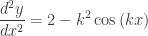
The question showed the three figures below and identified figure 1 as the graph of $f\left( x \right)={{x}^{2}}$ and figure 2 as the graph of $g\left( x \right)=\cos \left( x \right)$ . The question then allowed as how one might think of the graph is figure 3 as the graph of $h\left( x \right)={{x}^{2}}+\cos \left( x \right)$ , the sum of these two functions. Not that unreasonable an assumption, but apparently not correct.

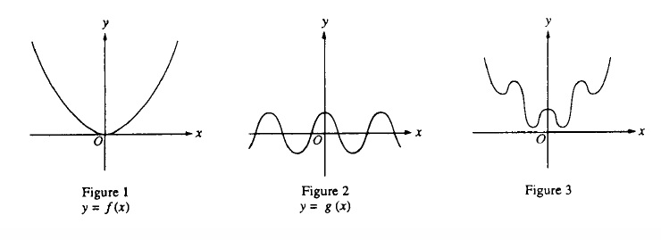
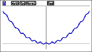
Part a: The students first were asked to sketch the graph of $h\left( x \right)$ in a window with [–6, 6] x [–6, 40] (given this way). A box with axes was printed in the answer booklet. This was a calculator required question and the result on a graphing calculator looks like this:

$y={{x}^{2}}+\cos \left( x \right)$ .
The window is [-6,6] x [-6, 40]

Students were expected to copy this onto the answer page. Note that the graph exits the screen below the top corners and it does not go through the origin. Both these features had to be obvious on the student’s paper to earn credit.

Part b: The second part of the question instructed students to use the second derivative of $h\left( x \right)$ to explain why the graph does not look like figure 3.

$\displaystyle \frac{dy}{dx}=2x-\sin \left( x \right)$

$\displaystyle \frac{{{d}^{2}}y}{d{{x}^{2}}}=2-\cos \left( x \right)$

Students then had to observe that the second derivative was always positive (actually it is always greater than or equal to 1) and therefore the graph is concave up everywhere. Therefore, it cannot look like figure 3.

Part c: The last part of the question required students to prove (yes, “prove”) that the graph of $y={{x}^{2}}+\cos \left( kx \right)$ either had no points of inflection or infinitely many points of inflection, depending on the value of the constant k.

Successful student first calculated the second derivative:

$\displaystyle \frac{dy}{dx}=2x-k\sin \left( kx \right)$

$\displaystyle \frac{{{d}^{2}}y}{d{{x}^{2}}}=2-{{k}^{2}}\cos \left( kx \right)$

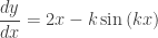
Then considering the sign of the second derivative, if ${{k}^{2}}\le 2$ , $\frac{{{d}^{2}}y}{d{{x}^{2}}}\ge 0$ and there are no inflection points (the graph is always concave up). But, if ${{k}^{2}}>2$ , then since y” is periodic and changes sign, it does so infinitely many times and there are then infinitely many inflection points. See the figure below.

k = 8

Using this question as a class exercise

Notice how the question leads the student in the right direction. If they go along with the problem they are going in the right direction. In class, I would be inclined to make them work for it.

First, I would ask the class if figure 3 is the correct graph of $h\left( x \right)={{x}^{2}}+\cos \left( x \right)$ . I would let them, individually, in groups, or as a class suggest and defend an answer. I would not even suggest, but certainly not mind, if they used a graphing calculator.
Once they determined the correct answer, I would ask them to justify (or prove) their conjecture. Again, no hints; let the class struggle until they got it. I may give them a hint along the lines of what does figure 3 have or do that the correct graph does not. (Answer: figure 3 changes concavity). Sooner or later someone should decide to check out the second derivative.
Then I’d ask what could be the equation for a graph that does look like figure 3. You could give hints along the line of changing the coefficients of the terms of the second derivative. There are several ways to do this and all are worth considering.
1. Changing the coefficient of the x² term (to a proper fraction, say, 0.02) will do the trick. If that’s what they come up with fine – it’s correct.
2. If you want to be picky, this causes the graph to go negative and figure 3 does not do that, but I ‘d let that go and ask if changing the coefficient of the cosine term in the second derivative can be done and if so how do you do that.
3. This may be done by simply putting a number in front of the cosine term of the original function, say $h\left( x \right)={{x}^{2}}+6\cos \left( x \right)$ , but the results really do not look like figure 3,
4. If necessary, give them the hint $y={{x}^{2}}+\cos \left( kx \right)$

1995 was the first year graphing calculators were required on the AP Calculus exams. They were allowed for all questions, but most questions had no place to use them. The parametric equation question on the same test, 1995 BC 1, was also a good question that made use of the graphing capability of calculators to investigate the relative motion of two particles in the plane. The AB Exam in 1995 only required students to copy one graph from their calculator.

Both BC questions were generally well received at the reading. I know I liked them. I was looking forward to more of the same in coming years.

I was disappointed.

There was an attempt the following year (1997 AB4/BC4), but since then nothing investigating families of functions (i.e. like these with a parameter that affects the shape of the graph) or anything similar has appeared on the exams. I can understand not wanting to award a lot of points for just copying the graph from your calculator onto the paper, but in a case like this where the graph leads to a rich investigation of a counterintuitive situation I could get over my reluctance.

But that’s just me.

Power Rule Implies Chain Rule

Posted on September 20, 2014 by Lin McMullin

Having developed the Product Rule $d\left( uv \right)=u{v}'+{u}'v$ and the Power Rule $\frac{d}{dx}{{x}^{n}}=n{{x}^{n-1}}$ for derivatives in your class, you can explore similar rules for the product of more than two functions and suddenly the Chain Rule will appear.

For three functions use the associative property of multiplication with the rule above:

$d\left( uvw \right)=d\left( \left( uv \right)w \right)=u\cdot v\cdot dw+w\cdot d(uv)=u\cdot v\cdot dw+w\left( udv+vdu \right)$

So expanding with a slight change in notation:

$d\left( uvw \right)=uv{w}'+u{v}'w+u'vw$

For four factors there is a similar result:

$d\left( uvwz \right)=uvw{z}'+uv{w}'z+u{v}'wz+{u}'vwz$

Exercise: Let ${{f}_{i}}$ for $i=1,2,3,...,n$ be functions. Write a general formula for the derivative of the product ${{f}_{1}}{{f}_{2}}{{f}_{3}}\cdots {{f}_{n}}$ as above and in sigma notation

Answers

$d\left( {{f}_{1}}{{f}_{2}}{{f}_{3}}\cdots {{f}_{n}} \right)={{f}_{1}}{{f}_{2}}{{f}_{3}}\cdots {{{f}'}_{n}}+{{f}_{1}}{{f}_{2}}{{{f}'}_{3}}\cdots {{f}_{n}}+{{f}_{1}}{{{f}'}_{2}}{{f}_{3}}\cdots {{f}_{n}}+\cdots +{{{f}'}_{1}}{{f}_{2}}{{f}_{3}}\cdots {{f}_{n}}$

$\displaystyle d\left( {{f}_{1}}{{f}_{2}}{{f}_{3}}\cdots {{f}_{n}} \right)=\sum\limits_{i=1}^{n}{\frac{{{f}_{1}}{{f}_{2}}{{f}_{3}}\cdots {{f}_{n}}}{{{f}_{i}}}{{{{f}'}}_{i}}}$

This idea may now be used to see the Chain Rule appear. Students may guess that $d{{\left( f \right)}^{4}}=4{{\left( f \right)}^{3}}$ , but wait there is more to it.

Write ${{\left( f \right)}^{4}}=f\cdot f\cdot f\cdot f\text{ }$ . Then from above

$d{{\left( f \right)}^{4}}=d\left( f\cdot f\cdot f\cdot f\text{ } \right)=f\cdot f\cdot f\cdot {f}'+f\cdot f\cdot {f}'\cdot f+f\cdot {f}'\cdot f\cdot f+{f}'\cdot f\cdot f\cdot f$

$d{{\left( f \right)}^{4}}=4{{\left( f \right)}^{3}}{f}'\text{ }$

Looks just like the power rule, but there’s that “extra” ${f}'$ . Now you are ready to explain about the Chain Rule in the next class.

Mean Tables

Posted on September 16, 2014 by Lin McMullin

The AP calculus exams always seem to have a multiple-choice table question in which the stem describes function in words and students are asked which of 5, now 4, tables could be a table of values for the function. Could be because you can never be sure without other information what happens between values in the table. So, the way to solve the problem is to eliminate choices that are at odds with the description.

The question style nicely makes students relate a verbal description with the numerical information in the tables. This uses two parts of the Rule of Four.

In 2003, question AB 90 told students that a function f had a positive first derivative and a negative second derivative on the closed interval [2, 5]. There were five tables to choose from.

There is a fairly quick way to solve the problem, but I want to go a little slower and discuss the theorems that apply.

First, since the function has first and second derivatives on the interval, the function and its first derivative are continuous on the interval. This is important since, if they were not continuous, there would be no way to solve the problem.

Next, since the first derivative is positive, the function must be increasing. This allowed students to quickly eliminate three choices where the function was obviously decreasing. The remaining tables showed increasing values and thus could not be eliminated based on the first derivative.

The two remaining tables were

Notice that in table A the values are increasing at an increasing rate, and in table B the values are increasing at a decreasing rate. Thus, table B is the correct choice. By the end of the year that kind of reasoning is enough for students to determine the correct answer.

Students could also draw a quick graph and see that table A was concave up and B was concave down. This will give them the correct answer, but technically it is a wrong approach since, once again, there is no way to know what happens between the values; we should not just connect the points and draw a conclusion.

The correct reasoning is based on the Mean Value Theorem (MVT).

In table A, by the MVT there must be a number c₁ between 2 and 3 where ${f}'\left( {{c}_{1}} \right)=2$ the slope between the points (2,7) and (3, 9). Also, there must be a number c₂ between 3 and 4 where ${f}'\left( {{c}_{2}} \right)=3$ the slope between (3, 9) and (4, 12), and likewise a number c₃ between 4 and 5 where ${f}'\left( {{c}_{3}} \right)=4$ .

Then applying the MVT to these values of ${f}'\left( x \right)$ , there must be a number, say d₁ between c₁ and c₂ where ${{f}'}'\left( {{d}_{1}} \right)=\frac{3-2}{{{c}_{2}}-{{c}_{1}}}>0$ . Since the second derivative should be negative everywhere, table A is eliminated making the remaining table B the correct choice.

If we do a similar analysis of Table B, we find that the MVT values for the second derivative are all negative. However, we cannot be sure this is true for all values of f in table B, since we can never be sure what happens between the values in a table. But table B is the only one that could be the one described since the others clearly are not.

In this post we saw how the MVT can be used in a numerical setting. I discussed the MVT in an analytic setting on September 28, 2012 and graphically on October 1, 2012.

Darboux’s Theorem

Posted on August 18, 2014 by Lin McMullin

Jean Gaston Darboux
1842 – 1917

Jean Gaston Darboux was a French mathematician who lived from 1842 to 1917. Of his several important theorems the one we will consider says that the derivative of a function has the Intermediate Value Theorem property – that is, the derivative takes on all the values between the values of the derivative at the endpoints of the interval under consideration.

Darboux’s Theorem is easy to understand and prove but is not usually included in a first-year calculus course (and is not included on the AP exams). Its use is in the more detailed study of functions in a real analysis course.

You may want to use this as an enrichment topic in your calculus course, or a topic for a little deeper investigation. The ideas here are certainly within the range of what first-year calculus students should be able to follow. They relate closely to the Mean Value Theorem (MVT). I will suggest some ideas (in blue) to consider along the way.

More precisely Darboux’s theorem says that

If f is differentiable on the closed interval [a, b] and r is any number between f ’ (a) and f ’ (b), then there exists a number c in the open interval (a, b) such that f ‘ (c) = r.

Differentiable on a closed interval?

Most theorems in beginning calculus require only that the function be differentiable on an open interval. Here, obviously, we need a closed interval so that there will be values of the derivative for r to be between.

The limit definition of derivative requires a regular two-sided limit to exist; at the endpoint of an interval there is only one side. For most theorems this is enough. Here the definition of derivative must be extended to allow one-sided limits as x approaches the endpoint values from inside the interval. Also note that if a function is differentiable on (a, b), then it is differentiable on any closed sub-interval of (a, b) that does not include a or b.

Geometric proof [1]

Consider the diagram below, which shows a function in blue. At each endpoint draw a line with the slope of r. Notice that these two lines have a slope less than that of the function at the left end and greater than the slope at the right end. At least one of these lines must intersect the function at an interior point of the interval. Before reading on, see if you and your students can complete the proof from here. (Hint: What theorem does the top half of the figure remind you of?)

On the interval between the intersection point and the end point we can apply the Mean Value Theorem and determine the value of c where the tangent line will be parallel to the line through the endpoint. At this point f ‘(c) = r. Q.E.D.

Analytic Proof [2]

Consider the function $h\left( x \right)=f\left( x \right)-(f(b)+r(x-b))$ . Since f(x) is differentiable, it is continuous; $\displaystyle f(b)+r(x-a)$ is also continuous and differentiable. Therefore, h(x) is continuous and differentiable on [a, b]. By the Extreme Value Theorem, there must be a point, x = c, in the open interval (a, b) where h(x) has an extreme value. At this point h’ (c) = 0.

Before reading on see if you can complete the proof from here.

$\displaystyle h(x)=f(x)-(f(b)+r(x-a))$

$\displaystyle {h}'(x)={f}'(x)-r$

$\displaystyle {h}'(c)={f}'(c)-r=0$

$\displaystyle {f}'\left( c \right)=r$

Q.E.D.

Exercise: Compare and contrast the two proofs.

In the geometric proof, what does $\displaystyle y=f(b)+r(x-a)$ represent? Where does it show up in the diagram?
How do both proofs relate to the Mean Value Theorem (or Rolle’s Theorem).

The function $\displaystyle h(x)=f(x)-(f(b)+r(x-a))$ represents the vertical distance from f(x) to $\displaystyle f(b)+r(x-a)$ . In the diagram, this is a vertical segment connecting f(x) to $\displaystyle y=f(b)+r(x-a)$ .This expression may be positive, negative, or zero. In the diagram, at the point(s) where the line through the right endpoint intersects the curve and at the endpoint h(x) = 0. Therefore, h(x) meets the hypotheses of Rolle’s Theorem (and the MVT), and the result follows.

The line through the right endpoint will have equation the $y=f(b)+r(x-b)$ This makes $h\left( x \right)=f\left( x \right)-\left( f(b)+r(x-b) \right)$ . When differentiated and the result will be ${f}'\left( x \right)-r$ the same expression as in the analytic proof.

Also, you may move this line upwards parallel to its original position and eventually it will be tangent to the graph of the function. (See my posts on MVT 1 and especially MVT 2).

Exercise:

Consider the function f(x) = sin(x)

On the interval [1,3] what values of the derivative of f are guaranteed by Darboux’s Theorem? .
Does Darboux’s theorem guarantee any value on the interval $[0,2\pi ]$ ? Why or why not?

Answers:

f ‘(x) = cos(x). f ‘ (1) = 0.54030 and f ‘ (3) = -0.98999. So the guaranteed values are from -0.98999 to 0.54030.
No. f ‘ (x) = 1 at both endpoints, so there are no values between one and one.

Another interesting aspect of Darboux’s Theorem is that there is no requirement that the derivative f ‘(x) be continuous!

A common example of such a function is

$\displaystyle f\left( x \right)=\left\{ \begin{matrix} {{x}^{2}}\sin \left( \frac{1}{x} \right) & x\ne 0 \\ 0 & x=0 \\ \end{matrix} \right.$

With $\displaystyle {f}'\left( x \right)=-\cos \left( \tfrac{1}{x} \right)+2x\sin \left( \tfrac{1}{x} \right),\,\,x\ne 0$ .

This function (which has appeared on the AP exams) is differentiable (and therefore continuous).There is an oscillating discontinuity at the origin. The derivative is not continuous at the origin. Yet, every interval containing the origin as an interior point meets the conditions of Darboux’s Theorem, so the derivative while not continuous has the intermediate value property.

AP exam question 1999 AB3/BC3 part c:

Finally, what inspired this post was a recent discussion on the AP Calculus Community bulletin board about the AP exam question 1999 AB3/BC3 part c. This question gave a table of values for the rate, R, at which water was flowing out of a pipe as a differentiable function of time t. The question asked if there was a time when R’ (t) = 0. It was expected that students would use Rolle’s Theorem or the MVT. There was a discussion about using Darboux’s theorem or saying something like the derivative increased (or was positive), then decreased (was negative) so somewhere the derivative must be zero (implying that derivative had the intermediate value property). Luckily, no one tried this approach, so it was a moot point.

Take a look at the problem with your students and see if you can use Darboux’s theorem. Be sure the hypotheses are met.

Answer (try it yourself before reading on):

The function is not differentiable at the endpoints. But consider an interval like [0,3]. Using the given values in the table, by the MVT there is a time t = c where R‘(c) = 0.8/3 > 0, and there is a time t = d on the interval [21, 24] where R‘(d) = -0.6/3 < 0. The function is differentiable on the closed interval [c, d] so by Darboux’s Theorem there must exist a time when R’(t) = 0. Admittedly, this is a bit of overkill.

References:

After Nitecki, Zbigniew H. Calculus Deconstructed A Second Course in First-Year Calculus, ©2009, The Mathematical Association of America, ISBN 978-0-883835-756-4, p. 221-222.
After Dunham, William The Calculus Gallery Masterpieces from Newton to Lebesque, © 2005, Princeton University Press, ISBN 978-0-691-09565-3, p. 156.

Both these book are good reference books.

Updated: August 20, 2014, and October 4, 2017

Implicit Differentiation of Parametric Equations

Posted on May 17, 2014 by Lin McMullin

I’ve never liked memorizing formulas. I would rather know where they came from or be able to tie it to something I already know. One of my least favorite formulas to remember and explain was the formula for the second derivative of a curve given in parametric form. No longer.

If $y=y\left( t \right)$ and, $x=x\left( t \right)$ then the tradition formula gives

$\displaystyle \frac{d}{dx}y\left( t \right)=\frac{dy/dt}{dx/dt}$ , and

$\displaystyle \frac{{{d}^{2}}y}{d{{x}^{2}}}=\frac{\frac{d}{dt}\left( \frac{dy}{dx} \right)}{\frac{dx}{dt}}$

It is that last part, where you divide by $\displaystyle \frac{dx}{dt}$ , that bothers me. Where did the $\displaystyle \frac{dx}{dt}$ come from?

Then it occurred to me that dividing by $\displaystyle \frac{dx}{dt}$ is the same as multiplying by $\displaystyle \frac{dt}{dx}$

It’s just implicit differentiation!

Since $\displaystyle \frac{dy}{dx}$ is a function of t you must begin by differentiating the first derivative with respect to t. Then treating this as a typical Chain Rule situation and multiplying by $\displaystyle \frac{dt}{dx}$ gives the second derivative. (There is a technical requirement here that given $x=x\left( t \right)$ , then $t={{x}^{-1}}\left( x \right)$ exists.)

In fact, if you look at a proof of the formula for the first derivative, that’s what happens there as well:

$\displaystyle \frac{d}{dx}y\left( t \right)=\frac{dy}{dt}\cdot \frac{dt}{dx}=\frac{dy/dt}{dx/dt}$

The reason you to do it this way is that since x is given as a function of t, it may be difficult to solve for t so you can find dt/dx in terms of x. But you don’t have to; just divide by dx/dt which you already know.

Here is an example for both derivatives.

Suppose that $x={{t}^{3}}-3$ and $y=\ln \left( t \right)$

Then $\displaystyle \frac{dy}{dt}=\frac{1}{t}$ , and $\displaystyle \frac{dx}{dt}=3{{t}^{2}}$ and $\displaystyle \frac{dt}{dx}=\frac{1}{3{{t}^{2}}}$ .

Then $\displaystyle \frac{dy}{dx}=\frac{1}{t}\cdot \frac{dt}{dx}=\frac{1}{t}\cdot \frac{1}{3{{t}^{2}}}=\frac{1}{3{{t}^{3}}}=\frac{1}{3}{{t}^{-3}}$

And $\displaystyle \frac{{{d}^{2}}y}{d{{x}^{2}}}=\left( \frac{d}{dt}\left( \frac{dy}{dx} \right) \right)\cdot \frac{dt}{dx}=\left( -{{t}^{-4}} \right)\cdot \frac{dt}{dx}=\left( -{{t}^{-4}} \right)\left( \frac{1}{3{{t}^{2}}} \right)=-\frac{1}{3{{t}^{6}}}$

Yes, it’s the same thing as using the traditional formula, but now I’ll never have to worry about forgetting the formula or being unsure how to explain why you do it this way.

Revised: Correction to last equation 5/18/2014

Revised: 2/8/2016

Foreshadowing the Chain Rule

Posted on September 20, 2013 by Lin McMullin

I assigned another very easy but good problem this week. It was simple enough, but it gave a hint of things to come.

Use the Product Rule to find the derivative of ${{\left( f\left( x \right) \right)}^{2}}$ .

Since we have not yet discussed the Chain Rule, the Product Rule was the only way to go.

$\frac{d}{dx}{{\left( f \right)}^{2}}=\frac{d}{dx}\left( f\cdot f \right)=f\cdot {f}'+{f}'\cdot f=2f\cdot f'$

And likewise for higher powers:

$\frac{d}{dx}{{f}^{3}}=\frac{d}{dx}\left( f\cdot f\cdot f \right)=f\cdot f\cdot {f}'+f\cdot {f}'\cdot f+{f}'\cdot f\cdot f=3{{f}^{2}}{f}'$

If you just look at the answer, it is not clear where the ${f}'$ comes from. But the result foreshadows the Chain Rule.

Then we used the new formula to differentiate a few expressions such as ${{\left( 4x+7 \right)}^{2}}$ and ${{\sin }^{2}}\left( x \right)$ and a few others.

Regarding the Chain Rule: I have always been a proponent of the Rule of Four, but I have never seen a good graphical explanation of the Chain Rule. (If someone has one, PLEASE send it to me – I’ll share it.)

Here is a rough verbal explanation that might help a little.

Consider the graph of $y=\sin \left( x \right)$ . On the interval $[0,2\pi ]$ it goes through all its value in order once – from 0 to 1 to 0 to -1 and back to zero. Now consider the graph of $y=\sin \left( 3x \right)$ . On the interval $\left[ 0,\tfrac{2\pi }{3} \right]$ it goes through all the same values in one-third of the time. Therefore, it must go through them three times as fast. So the rate of change of $y=\sin \left( 3x \right)$ between 0 and $\tfrac{2\pi }{3}$ must be three times the rate of change of $y=\sin \left( x \right)$ . So the rate of change of must be $3\cos \left( 3x \right)$ . Of course this rate of change is the slope and the derivative.

At Just the Right Time

Posted on September 12, 2013 by Lin McMullin

This is about a little problem that appeared at just the right time. My class had just learned about derivatives (limit definition) and the fact that the derivative is the slope of the tangent line. But none of that was really firm yet. I had assigned this problem for homework:¹

Find f (3) and f ‘ (3), assuming that the tangent line to y = f (x) at a = 3 has equation y = 5x + 2

To solve the problem, you need to realize that the tangent line and the function intersect at the point where x = 3. So, f (3) was the same as the point on the line where x = 3. Therefore, f (3) = 5(3) + 2 = 17.

Then you have to realize that the derivative is the slope of the tangent line, and we know the tangent line’s equation and we can read the slope. So f ‘ (3) = 5

In my previous retired years, I wrote a number of questions for several editions of a popular AP Calculus exam review book.² I found it easy to write difficult questions. But what I was after was good easy questions; they are more difficult to write. One type of good easy question is one that links two concepts in a way that is not immediately obvious such as the question above. I am always amazed at the good easy questions on the AP calculus exams. Of course, they do not look easy, but that’s what makes them good.

Now a month from now this question will not be a difficult at all – in fact it did not stump all of my students this week. Nevertheless, appearing at just the right time, I think it did help those it did stump, and that’s why I like it.

______________________

² These review books are published by D&S Marketing Systems, Inc. Website

Teaching Calculus

The pleasure lies not in discovering the truth, but in searching for it.

Category Archives: Derivative Theory

Good Question 3 1995 BC 5

Power Rule Implies Chain Rule

Mean Tables

Darboux’s Theorem

Implicit Differentiation of Parametric Equations

Foreshadowing the Chain Rule

At Just the Right Time

Share this:

Share this:

Share this:

Share this:

Share this:

Share this:

Share this: