
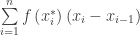
In our last post we discussed what are called Riemann sums. A sum of the form 

The three most common are these and depend on where the 
- Left-Riemann sum, L, uses the left side of each sub-interval, so
.
- Right-Riemann sum, R, uses the right side of each sub-interval, so
.
- Midpoint-Riemann sum, M, uses the midpoint of each interval, so
.
For the AP Exams students should know these and be able to compute them. The actual values are often given in a table, so the long computation of the function values is not necessary.
Another way of approximating the area between the graph and the x-axis is to use trapezoids formed by joining the points at the ends of each sub-interval. The areas can be figured individually and added or the value, T, can be found by averaging the left- and right-Riemann sums, 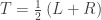
Whenever you are dealing with approximations, you should have some sense of how good they are. All of the approximations discussed will get closer to the true area if more values (more partition points) are used.
If the graph is increasing on the interval, then the left-sum is an underestimate of the actual value and the right-sum is an overestimate. If the curve is decreasing, then the right-sums are underestimates and the left-sums are overestimates. (To see why, draw a sketch.)
If the graph is concave up the trapezoid approximation is an overestimate, and the midpoint is an underestimate. If the graph is concave down, then trapezoids give an underestimate and the midpoint an overestimate. (To see how this works, draw a sketch. For the midpoint draw the tangent line at the midpoint to the sides of the sub-interval; this trapezoid has the same area as the rectangle drawn at the midpoint of the interval. Why?)
If the graphs are not monotone on the interval or change concavity, then all bets are off.
For all of the Riemann sums, including those not mentioned above, as the number of partition points increase (

Corrected 11-28-2017
 .
. . This is called a partition of the interval. The x-coordinates are
  ,
, 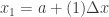 ,
, 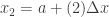 ,
,  up to
up to 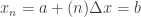 .
. , which may be a little complicated. If you decide on using the right end then for the ith sub-interval
 ![[{{x}_{i-1}},{{x}_{i}}]](https://s0.wp.com/latex.php?latex=%5B%7B%7Bx%7D_%7Bi-1%7D%7D%2C%7B%7Bx%7D_%7Bi%7D%7D%5D&bg=ffffff&fg=333333&s=0&c=20201002) the value is
the value is  , for the left side the value is
  . This is the vertical distance between the graph and the x-axis.
 . Do this for each sub-interval and add the results to get your approximation. For the right side approximation this looks like
  .
. .
.
 . This is correct only if f (x) > 0. There is a natural confusion for beginning students between the facts that if f (x) < 0 the integral comes out negative, but the area is positive.
 which is positive as it should be. And students will immediately see that
