
Applications of Integration 1 – Area Between Curves
The first thing to keep in mind when teaching the applications of integration is Riemann sums. The thing is that when you set up and solve the majority of application problems you cannot help but develop a formula for the situation. Students think formulas are handy and go about memorizing them badly. By which I mean they forget or never learn where the various things in the formula come from. A slight change in the situation and they are lost. Behind every definite integral stands a Riemann sum; each application should be approached through its Riemann sum. If students understand that, they will make fewer mistakes with the “formula.”
As I suggested in a previous post, I believe all area problems should be treated as the area between two curves. If you build the Riemann sum rectangle between the graph and the axis and calculate its vertical side as the upper function minus the lower (or right minus left if you use horizontal rectangles) you will always get the correct integral for the area. If the upper curve is the x-axis, then the vertical sides of the Riemann sums are (0 – f(x)) and you get a positive area as you should.
If both your curves are above the x-axis, then it is tempting to explain what you are doing as subtracting the area between the lower curve and the x-axis from the area between the upper curve and the x-axis. And this is not wrong. It just does not work very smoothly when one, both or parts of either are below the x-axis. Then you go into all kinds of contortions explaining things in terms of positive and negative areas. Why go there?
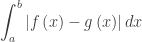
Regardless of where the two curves are relative to the x-axis, the vertical distance between them is the upper value minus the lower, f(x) – g(x). It does not matter if one or both functions are negative on all or part of the interval, the difference is positive and the area between them is

Furthermore, this Riemann sum rectangle is used in other applications. It is the one rotated in both the washer and shell method of finding volumes. So in area and all applications be sure your students don’t just memorize formulas, but keep their eyes on the rectangle and the Riemann sum.
Finally, if the graphs cross in the interval so that the upper and lower curves change place, you may (1) either break the problem into several pieces so that your integrands are always of the form upper minus lower, or (2) if you intend to do the computation using technology, set up the integral as
 .
.

 .
.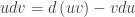 .
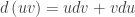
. . By the FTC the first term on the right can be simplified giving the formula for Integration by Parts:
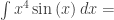
 in which there is a combination of functions that are usually of different types – here a polynomial and a trig function.
 . Here we make the substitutions
  and from these we compute
  . (There is no need for the +C here; it will be included later). Making these substitutions gives

 and
and  the result is
 . This is important because when evaluating definite integrals this allows us to do them term by term.
 . To see this make a quick table for the area between F(t) = t and compare it to the area functions for F2(t) = 2t.
 . Now use those numbers and the property in paragraph 3 to show that
  .
. regardless of the order of a ,b and c. The only thing that matters is that (1) the lower limit in the first integral on the left is the lower limit on the right, (2) the upper limit on the last integral on the left is the upper limit on the right, and (3) on the left the upper limit on one integral is the lower limit on the next. You can even string more integrals together as long as you follow the pattern.
 on the interval [a, b], then
  . This is sometimes called the “Racetrack Principle.” Interpreting f and g as rates and their integrals as amounts (or distances), then in the same interval, the faster horse travels farther.
 .
.
 ?
?
 ,
,
 to
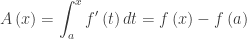
to  . What is the net change in f over this interval? Easy it’s
  . No problem, but way too easy for a calculus class. So let’s try a harder way!
 .
. .
. part. What to do?
 or
or  .
.
 .
. .
. .
. on the interval [1, 4]. Hover and click on the figure below.
