Adapting 2021 BC 6

Nine of nine. We continue our look at the 2021 free-response questions. We will look at ways to adapt, expand, and explore this question to help students better understand it and look at other questions that can be asked based on a similar stem.

2021 BC 6

This is a Sequence and Series (Type 10) question. Typically the topic of the last question on the BC exam, it tests the concepts in Unit 10 of the current Calculus Course and Exam Description. This year the previous question, 2021 BC 5, asked students to write a Taylor Polynomial. This question covers other related topics: convergence tests, radius of convergence, and the error bound.

There is a nuance here. In past years students were not asked to give the conditions for a convergence test and were expected to determine which test to use for themselves. I think the idea here, and perhaps going forward (?), is to make sure the students have considered the conditions necessary to use a test. This is in keeping with other questions where the hypotheses of the theorem students were using had to be checked (Cf. recent L’Hospital’s Rule questions).

The Convergence Test Chart  and the posts “Which Convergence Test Should I use?” Part 1 and Part 2 may be helpful.

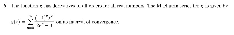
The stem for 2021 BC 6 is:

Part (a): Students were asked to give the conditions for the integral test and use it to determine if a different series, \sum\limits_{{n=0}}^{\infty }{{\frac{1}{{{{e}^{n}}}}}} converges.

Discussion and ideas for adapting this question:

  • Be sure your students know the conditions necessary for each convergence test. Phrase your questions as this one is phrased – at least sometimes.
  • Ask students to state the conditions for any convergence they use.
  • Discuss which tests (often plural) can be used for each series you study.
  • Make sure students can decide for themselves which test to use in case next year’s questions do not tell them.
  • Ask what other test(s) may be used with this series (Hint: the series is geometric). This is a question to ask for any series you study.

Part (b): Students are told to use the series from part (a) with the limit comparison test to show that the given series converges absolutely when x = 1. Again, students were asked to use a specific test. Notice that even if a student could not do part (a), they were not shut out of part (b).

Discussion and ideas for adapting this question:

  • Since you cannot count on being told which test to use for comparison, be sure to discuss how to decide which test(s) can be used with each series. Again see “Which Convergence Test Should I use?” Part 1 and Part 2.
  • Show students that proving absolute convergence is often a good way to eliminate the need for dealing with alternating series and other series with negative signs.

Part (c): Students were asked for the radius of convergence of the series. A standard question done by using the Ratio test.

Discussion and ideas for adapting this question:

The only extension here is to determine the interval of convergence, by checking the endpoints.

Part (d): Students were asked for the alternating series error bound using the first two terms to approximate the value of g(1). Even though there are only two error bounds students are expected to be able to compute (the other is the Lagrange error bound), students were again told which one to use. The result was not expected to be expressed as a decimal.

Discussion and ideas for adapting this question:

  • First, have students check that the conditions for using the alternating series error bound are met.
  • Increase the number of terms to be used.
  • Ask students to find the Lagrange error bound and compare the results.

This post on the series question concludes the series of posts (pun intended) considering how to expand and adapt the 2021 AP Calculus free-response questions. I hope you found them helpful.

As always, I happy to hear your ideas for other ways to use this question. Please share your thoughts and ideas.


Unit 1 – Limits and Continuity

This is a re-post and update of the first in a series of posts from last year. It contains links to posts on this blog about the topics of limits and continuity for your reference in planning. Other updated post on the 2019 CED will come throughout the year, hopefully, a few weeks before you get to the topic. 

Unit 1 contains topics on Limits and Continuity. (CED – 2019 p. 36 – 50). These topics account for about 10 – 12% of questions on the AB exam and 4 – 7% of the BC questions.

Logically, limits come before continuity since limit is used to define continuity. Practically and historically, continuity comes first. Newton and Leibnitz did not have the concept of limit the way we use it today. It was in the early 1800’s that the epsilon-delta definition of limit was first given by Bolzano (whose work was overlooked) and then by Cauchy, Jordan, and Weierstrass. But, their formulation did not use the word “limit”, rather the use was part of their definition of continuity. Only later was it pulled out as a separate concept and then returned to the definition of continuity as a previously defined term. See Which Came First?

Students should have plenty of experience in their math courses before calculus with functions that are and are not continuous. They should know the names of the types of discontinuities – jump, removable, infinite, oscillating etc.and the related terms such as asymptote. As you go through this unit, you may want to quickly review these terms and concepts as they come up.

(As a general technique, rather than starting the year with a week or three of review – which the students need but will immediately forget again – be ready to review topics as they come up during the year as they are needed – you will have to do that anyway. See Getting Started #2)

Topics 1.1 – 1.9: Limits

Topic 1.1: Suggests an introduction to calculus to give students a hint of what’s coming. See Getting Started #3

Topic 21.: Proper notation and multiple-representations of limits.

There is an exclusion statement noting that the delta-epsilon definition of limit is not tested on the exams, but you may include it if you wish. The epsilon-delta definition is not tested probably because it is too difficult to write good questions. Specifically, (1) the relationship for a linear function is always  delta =frac{varepsilon }{{left| m right|}}  where m is the slope and is too complicated to compute for other functions, and (2) for a multiple-choice question the smallest answer must be correct. (Why?)

Topic 1.3: One-sided limits.

Topic 1.4: Estimating limits numerically and from tables.

Topic 1.5: Algebraic properties of limits.

Topic 1.6: Simplifying expressions to find their limits. This can and should be done along with learning the other concepts and procedures in this unit.

Topic 1.7: Selecting the proper procedure for finding a limit. The first step is always to substitute the value into the limit. If this comes out to be number than that is the limit. If not, then some manipulation may be required. This can and should be done along with learning the other concepts and procedures in this unit.

Topic 1.8: The Squeeze Theorem is mainly used to determine  underset{{xto 0}}{mathop{{lim }}},frac{{sin left( x right)}}{x}=1 which in turn is used in finding the derivative of the sin(x). (See Why Radians?) Most of the other examples seem made up just for exercises and tests. (See 2019 AB 6(d)). Thus, important, but not too important.

Topic 1.9: Connecting multiple-representations of limit. This can and should be done along with learning the other concepts and procedures in this unit. Dominance, Topic 15, may be included here as well (EK LIM-2.D.5)

Topics 1.10 – 1.16 Continuity

Topic 1.10: Here you can review the different types of discontinuities with examples and graphs.

Topic 1.11: The definition of continuity. The EK statement does not seem to use the three-hypotheses definition. However, for the limit to exist and for f(c) to exist, they must be real numbers (i.e. not infinite). This is tested often on the exams, so students should have practice with verifying that (all three parts of) the hypothesis are met and including this in their answers.

Topic 1.12: Continuity on an interval and which Elementary Functions are continuous for all real numbers.

Topic 1.13: Removable discontinuities and handing piecewise – defined functions

Topic 1.14: Vertical asymptotes and unbounded functions. Here be sure to explain the difference between limits “equal to infinity” and limits that do not exist (DNE). See Good Question 5: 1998 AB2/BC2.

Topic 1.15: Limits at infinity, or end behavior of a function. Horizontal asymptotes are the graphical manifestation of limits at infinity or negative infinity. Dominance is included here as well (EK LIM-2.D.5)

Topic 1.16: The Intermediate Value Theorem (IVT) is a major and important result of a function being continuous. This is perhaps the first Existence Theorem students encounter, so be sure to stop and explain what an existence theorem is.


The suggested number of 40 – 50 minute class periods is 22 – 23 for AB and 13 – 14 for BC. This includes time for testing etc. If time seems to be a problem you can probably combine topics 3 – 5, topics 6 -7, topics 11 – 12. Topics 6, 7, and 9 are used with all the limit work.


There are three other important limits that will be coming in later Units:

The definition of the derivative in Unit 2, topics 1 and 2

L’Hospital’s Rule in Unit 4, topic 7

The definition of the definite integral in Unit 6, topic 3.

Posts on Continuity

CONTINUITY To help understand limits it is a good idea to look at functions that are not continuous. Historically and practically, continuity should come before limits. On the other hand, the definition of continuity requires knowing about limits. So, I list continuity first. The modern definition of limit was part of Weierstrass’ definition of continuity.

Which Came First? (7-28-2020)

Continuity (8-13-2012)

Continuity (8-21-2013) The definition of continuity.

Continuous Fun (10-13-2015) A fuller discussion of continuity and its definition

Right Answer – Wrong Question (9-4-2013) Is a function continuous even if it has a vertical asymptote?

Asymptotes (8-15-2012) The graphical manifestation of certain limits

Fun with Continuity (8-17-2012) the Diriclet function

Far Out! (10-31-2012) When the graph and dominance “disagree” From the Good Question series

Posts on Limits

Why Limits? (8-1-2012)

Deltas and Epsilons (8-3-2012) Why this topic is not tested on the AP Calculus Exams.

Finding Limits (8-4-2012) How to…

Dominance (8-8-2012) See limits at infinity

Determining the Indeterminate (12-6-2015) Investigating an indeterminate form from a differential equation. From the Good Question series.

Locally Linear L’Hôpital (5-31-2013) Demonstrating L’Hôpital’s Rule (a/k/a L’Hospital’s Rule)

L’Hôpital’s Rules the Graph (6-5-2013)

Unlimited


Here are links to the full list of posts discussing the ten units in the 2019 Course and Exam Description. the 2019 versions

2019 CED – Unit 1: Limits and Continuity

2019 CED – Unit 2: Differentiation: Definition and Fundamental Properties.

2019 CED – Unit 3: Differentiation: Composite , Implicit, and Inverse Functions

2019 CED – Unit 4 Contextual Applications of the Derivative  Consider teaching Unit 5 before Unit 4

2019 – CED Unit 5 Analytical Applications of Differentiation  Consider teaching Unit 5 before Unit 4

2019 – CED Unit 6 Integration and Accumulation of Change

2019 – CED Unit 7 Differential Equations  Consider teaching after Unit 8

2019 – CED Unit 8 Applications of Integration   Consider teaching after Unit 6, before Unit 7

2019 – CED Unit 9 Parametric Equations, Polar Coordinates, and Vector-Values Functions 

2019 CED Unit 10 Infinite Sequences and Series


Starting the Year

As you get ready to start school, here are some thoughts on the first week in AP Calculus. I looked back recently at some of the “first week of school” advice I offered in the past. Here’s a quick (actually, a bit longer then I planned) summary with some new ideas.

  1. The last time I taught AP Calculus during review time a student asked if there was a list of what’s on the exam. Duh! Why didn’t I think of that? So, I made copies of the list (from the old Acorn Book) and gave it to everyone. I should have done that on Day 1. So, my first suggestion is to make a copy of the “Mathematical Practices” and the “Course at a Glance” from the 2019 AP Calculus Course and Exam Description (p. 14 and p. 20 – 23) and give them to your students. Check off the topics as you do them during the year. 
  1. DON’T REVIEW! Yes, students have forgotten everything they ever learned in mathematics, but if you reteach it now, they will forget it again by the time they need it next week or next January. So, don’t waste the time, rather, plan to review material from Kindergarten thru pre-calculus when the topics come up during the year. Include short reviews in your lesson plans. For instance, when you study limits you will need to simplify rational expressions – that’s when you review rational expressions. When you look at the graphs of the trigonometric functions, that’s when to review the graphs of the parent functions, a lot of the terminology related to graphs, discontinuities, asymptotes, and even the values of the trigonometric functions of the special angles. Months from now you’ll be looking at inverse functions, that’s when you review inverses.
  1. In keeping with Unit 1 Topic 1, you may want to start with a brief introduction to calculus. Several years ago, when I first started this blog, Paul A. Foerster, was nice enough to share some preview problems. They give a taste of derivatives and integrals in the first week of school and get the kids into calculus right off the bat. Here is an updated version. Paul, who retired a few years ago after 50 (!) years of teaching, is Teacher Emeritus of Mathematics of Alamo High Heights School in San Antonio, Texas. He is the author of several textbooks including Calculus: Concepts and Applications. More information about the text and accompanying explorations can be found on the first page of the explorations. Thank you, Paul!
  1. If you are not already a member, I suggest you join the AP Calculus Community. We have over 18,000 members all interested in AP Calculus. The community has an active bulletin board where you can ask and answer questions about the courses. Teachers and the College Board also post resources for you to use. College Board official announcements are also posted here. I am the moderator of the community and I hope to see you there!
  1.  Here are some links to places on this blog that you may find helpful:
    1. Pacing– organizing your year.
    2. Check the Resource page from this blog.
    3. Calculator information:
    4. Miscellany: These posts discuss basic ideas that I always hoped students knew about mathematics before starting calculus

Adapting 2021 BC 6 the last in the series on adapting questions from the 2021 exam will appear in two weeks on Auguest 31, 2021


Revised August 16, 2021

Adapting 2021 BC 5

Eight of nine. We continue our study of the 2021 free-response questions. We will look at ways to adapt, expand, and explore this question to help students better understand it and look at other questions that can be asked based on a similar stem.

2021 BC 5

This is a Differential Equation (Type 6) with a Sequence and Series (Type 10) question included. It contains topics from Units 7 and 10 of the current Course and Exam Description (CED). It is not unusual for AP Calculus exam question to include several of the types in my classification and from several of the units from the CED (here units 7 and 10). In addition, the usual solving an initial value problem and a Euler’s Method approximation are included.

The stem for 2021 BC 5 is:

Part (a): Students were asked to write the second-degree Taylor polynomial for the function centered at x = 1 and then use it to approximate f(2). Students should stop after substituting 2 into their polynomial; no arithmetic or simplification is required, and a simplifying mistake will lose a point.

Discussion and ideas for adapting this question:

  • Ask students to find an expression for the second derivative (implicit differentiation).
  • Verify that \displaystyle {f}''\left( 1 \right)=4
  • Ask students to find the third-degree polynomial and use it to approximate f(2)

Part (b): Students were required to approximate f(2) using Euler’s method with two steps of equal size.

Discussion and ideas for adapting this question:

  • After you solve the equation in part (c), ask students to compare the approximations from parts (a) and (b) with the exact value. Neither approximation is very close to the exact value. Discuss why this is so. Consider the slope of the graph near x = 2.
  • Find a more accurate approximation using 3, 4, or more smaller steps. There are graphing calculator programs that will do the arithmetic. Do not hesitate to use them. Students have already shown they know how to do a Euler’s Method approximation; the point is to understand the situation.

Part (c): Finding the solution of the differential equation by separating the variables is expected in this kind of question. The added twist is that the method of integration by parts is necessary to find one of the antiderivatives.

 Discussion and ideas for adapting this question:

  • Be sure not to skip over removing the absolute value signs. The most efficient way is to realize that at (and near) the initial condition y > 0, so |y| = y. What do you do if y < 0?
  • There is not much you can do differently here. One thing is to change the initial condition. Try a negative value such as f(1) = –4.
  • As suggested in (b), compare, and discuss the approximations with the exact value.

Next week we will conclude this series of posts with a look at 2021 BC 6.

I would be happy to hear your ideas for other ways to use this question. Please use the reply box below to share your ideas.


Adapting 2021 BC 2

Seven of nine. This week we continue our look at the 2021 free-response questions with an eye to ways to adapt and expand the questions. Hopefully, you will find ways to use this and other free-response questions to help your students learn more and be better prepared for the exams.

2021 BC 2

This is a Parametric and Vector Equation (Type 8) question and contains topic from Unit 9 of the current Course and Exam Description. The vector equation of the velocity of a particle moving in the xy-plane is given along with the position of the particle at t = 0. No units were given.

The stem for 2021 BC 2 is next. (Note the \displaystyle \left\langle \text{ } \right\rangle notation for vectors. Any of the usual notations may be used by students, but be sure to show them the others in case the one their book usage is different than the exam’s.)

Part (a): Students were asked to find the speed and acceleration of the particle at t = 1.2. This is a calculator active questions and the students were expected, but not actually required, to use their calculator. With their calculator in parametric mode, students should begin by entering the velocity as xt1(t) and yt1(t).

Discussion and ideas for adapting this question:

  • There is little I can suggest here other than changing the time.
  • At the given time and other times, you can ask in what direction is the particle moving and which way the acceleration is pulling the velocity.
  • Ask student to do this without using their calculator. The answer need not be simplified or expressed as a decimal.

Part (b): Asked the students to find the total distance traveled by the particle over a given the time interval. This must be done on a calculator. Be sure your students know how to enter the expression using the already entered values for xt1(t) and yt1(t). The calculator entry should look like this.

\displaystyle \int_{0}^{{1.2}}{{\sqrt{{{{{\left( {\text{xt}1(t)} \right)}}^{2}}+{{{\left( {\text{yt1}(t)} \right)}}^{2}}}}}}dt

Discussion and ideas for adapting this question:

  • Use different intervals.
  • Discuss the similarities with the number line distance formula. In linear motion, the distance is simply the integral of the absolute value of the velocity. Since \displaystyle \int_{a}^{b}{{\left| {v\left( t \right)} \right|}}dt=\int_{a}^{b}{{\sqrt{{{{{\left( {v(t)} \right)}}^{2}}}}}}dt, this is the same formula reduced to one dimension.

Part (c): The situation is reduced to a one-dimensional problem: students were asked to find the coordinates of the point at which the particle is farthest left and explain why there is no point farthest to the right.

Discussion and ideas for adapting this question:

  • Discuss how to do this and how students should present their answer and explanation.
  • Show that this is the same as an extreme value problem and done the same way (i.e., find where the derivative is zero, and show that this is a minimum (farthest left), etc.).
  • Discuss how you know there is no maximum and interpret this in the context of the equation.

For further exploration. Try graphing the path of the particle. Discuss how to do that with your class. See what they suggest. Here a few approaches.

  • The first thought may be to integrate the velocity vector as an initial value problem. Unfortunately, this cannot be done. Neither the x-component nor the y-component can be integrated in terms of Elementary Functions. Even WolframAlpha.com is no help.
  • Having entered the velocity vector as xt1(t) and yt1(t), as suggested above, enter something like this depending on your calculator’s syntax and then graph in a suitable window. Compare the graph with the previous analysis in part (c)?

\displaystyle \text{x2t}(t)=-2+\int_{0}^{t}{{\text{x1t}(t)dt}}

\displaystyle \text{y2t}(t)=5+\int_{0}^{t}{{\text{y2t}(t)dt}}

  • You may also try expressing the components of velocity as a Taylor series centered at some positive number, a, not at zero. Integrate that to get an approximation to graph. Be sure to adjust things so the initial point is on the graph. WolframAlpha will help here. The one problem here is that the y-component is not defined for negative numbers. Therefore, zero cannt be then center and the largest the interval of convergence can be is [0, 2a] (Why?) and may not even by that large. This is an interesting approach mathematically but will not help with most of the graph.

Personal opinion: I do not think much of this question because all the first two parts require is entering the formula in your calculator and computing the answer, and the third part is really an AB level question. Just my opinion.


Seven of Nine

Next week 2021 BC 5

I would be happy to hear your ideas for other ways to use this question. Please use the reply box below to share your ideas.


Adapting 2021 AB 6

Six of nine. Continuing the current series of posts, this post looks at the AB Calculus 2021 exam question AB 6. Like most of the AP Exam questions, there is a lot more you can ask based on the stem of this question and a lot of other calculus you can discuss. This series of post offers suggestions as to how to adapt, expand, and use this question to help your students dig deeper and learn more.

2021 AB 6

This is a standard Differential Equation (Type 6) question and contains topics mainly from Unit 7 (Differential equations) and a little from Unit 3 (implicit differentiation) of the current Course and Exam Description. A differential equation with an initial condition is given in a context. The main part is the solution of the initial value question with three short other questions included.

The stem for 2021 AB 6 is:

Part (a): A slope field in the first quadrant with no scale on either axis is given. Students are asked to sketch the solution curve starting at the initial condition, the point (0, 0).  (I prefer this kind of slope field question to those where students are given a few points and asked to sketch the slope field through them. No one draws slope field by hand; slope field drawn by computers are used to study the approximate shape of the solution and determine its interesting properties as is done here and in part (b)). When drawing slope fields, the sketch should extend to from one border to another and contain the initial condition point.

Discussion and ideas for adapting this question:

  • Have student sketch solution through one or more different points. Copy the slope field and add the initial condition point somewhere else.
  • Add an initial point above the horizontal asymptote.
  • Compare and contrast the solutions drawn through several points.
  • Ask what the horizontal segments (at y = 12) tells you in the context of the problem.

Part (b):  Students are given the limit at infinity for the as yet unknow solution and asked to interpret it in the context of the problem including units of measure.

Discussion and ideas for adapting this question:

  • Discuss why this is so.
  • Discuss how to determine the units of the function from the given information.
  • Discuss how to determine the units of the derivative from the given information.
  • Discuss how to determine the units of the derivative from the units of the function.
  • Discuss how to determine the units of the function from the units of the derivative.
  • Discuss whether the interpretation of the limit makes sense in the context of the question.

Part (c): Students are asked to solve the initial value question using the method of separation of variables.

Discussion and ideas for adapting this question:

  • Since separation of variables is the only method for solving a differential equation that students are responsible for knowing, there is not much you can do to adapt or change this question.
  • The initial condition may be substituted immediately after the integration is done the “+ C” is attached, or it may be done later after the expression is solved for y. Show students both method and discuss which is more efficient and which makes more sense to them.
  • Removing the absolute value signs is another place that may confuse students. While some textbooks suggest using a “ ± “ sign and deciding sign which to use later, the better way is to decide as soon as possible. Ask yourself is the expression enclose by the absolute value signs positive or negative near (at) the initial value. If positive, then the absolute value is replaced by the same expression (as in this question); if negative, then the expression is replaced by its opposite. Then complete the question from there.

Part (d): This part needs careful reading. Students are asked, for a slightly different differential equation, if the rate of change in the amount of medicine is increasing or decreasing at a given time. Therefore, students must find the rate of change of the rate of change (the given derivative): the derivative of the derivative (i.e., the second derivative of the function). This requires implicit differentiation of the derivative using the quotient rule.

Discussion and ideas for adapting this question:

  • The second derivative has the first derivative as one of its factors. Students may (automatically) substitute the first derivative before simplifying or evaluating. This correct, but unnecessarily long. Show the students how to find and substitute the value of the first derivative along with the other numbers.
  • Do as little arithmetic as possible. You need only determine if the second derivative is positive or negative.
  • Discuss the meaning of the answer in the context of the problem.

Next week 2021 BC 2

I would be happy to hear your ideas for other ways to use this question. Please use the reply box below to share your ideas.


Adapting 2021 AB 5

Five of nine. Continuing the current series of posts, this post looks at the AB Calculus 2021 exam question AB 5. The series considers each question with the aim of showing ways to use the question in with your class as is, or by adapting and expanding it.  Like most of the AP Exam questions there is a lot more you can ask from the stem and a lot of other calculus you can discuss.

2021 AB 5

This question tests the process of differentiating an implicit function. In my scheme of type posts, it is in the Other Problems (Type 7) category; this type includes the topics of implicit functions, related rate problems, families of functions and a few others. This topic is in Unit 3 of the current Course and Exam Description. Every few exams one of these appears on the exams, but not often enough to be made into its own type.

The question does not lend itself to changes that emphasize the same concepts. Some of the suggestions below are for exploration beyond what is likely to be tested on the AP Exams.

Here is the stem, only one line long:

Part (a): Students were given dy/dx and asked to verify that the expression is correct. This is done so that a student who makes a mistake (or cannot find the derivative at all) will not be shut out of the rest of the question by not having the correct first derivative.

While not required for the exam, you could use a grapher in implicit mode to graph the relation. Without the y > 0 restriction the graph consists of two seemingly parallel graphs similar to a sine graph. They are not sine graphs.

Ideas for exploring this question:

  • Using a graphing utility that allows you to use sliders. Replace the -6 by a variable that will allow you to see all the members of this family using a slider.
  • If the slider value is between -1/8 and 0 the graph no longer looks the same. Explore with this.
  • If the slider value is < -1/8 there is no graph. Why?
  • Explain why these are not sine graphs. (Hint: Use the quadratic formula to solve for y):

\displaystyle y=\frac{{\sin (x)\pm \sqrt{{{{{(\sin (x))}}^{2}}+48}}}}{4}.

 Part (a): There is not much you can change in this part. Ask for the derivative of a different implicit relation. You may use other questions of this type. Good Question 17, 2004 AB 4, 2016 BC 4 (parts a, b, and c are suitable for AB).

Discussion and ideas for adapting this question:

  • Ask for the first derivative without showing student the answer.
  • Find the derivative from the expression when first solved for y. Show that this is equal to the given derivative.

Part (b): An easy, but important question: write the equation of the tangent line at a given point. Writing the equation of a line shows up somewhere on the exam every year. As always, use the point-slope form.

Discussion and ideas for adapting this question:

  • Use a different point.

Part (c): Students were asked to find the point in a specific interval where the tangent line is horizontal.

Discussion and ideas for adapting this question:

  • By enlarging the domain find other points where the tangent line is horizontal. (Not likely to be asked on the exam, but good exercise.)
  • Using y < 0 find where the tangent line is horizontal. (Not likely to be asked on the exam, but good exercise.)
  • Determine if the two parts of the graph are “parallel.”
  • Determine if the two parts of the graph are congruent to y=\tfrac{1}{4}\sin \left( x \right).

Part (d): Students were asked to determine if the point found in the previous part was a relative maximum, minimum or neither, and to justify their answer.  

Discussion and ideas for adapting this question:

  • Have students justify using the Candidates’ test (closed interval test).
  • Have students justify using the first derivative test.
  • Have students justify using the second derivative test.
  • Ask the same question for the branch with y < 0.

Having students justify local extreme values by all three methods is good practice any time there is a justification required. Depending on the problem, it may not be possible to use all three. Discuss why; discuss how to decide which is the most efficient for each problem.


Next week 2021 AB 6.

I would be happy to hear your ideas for other ways to use this question. Please use the reply box below to share your ideas.