At Just the Right Time

Posted on September 12, 2013 by Lin McMullin

This is about a little problem that appeared at just the right time. My class had just learned about derivatives (limit definition) and the fact that the derivative is the slope of the tangent line. But none of that was really firm yet. I had assigned this problem for homework:¹

Find f (3) and f ‘ (3), assuming that the tangent line to y = f (x) at a = 3 has equation y = 5x + 2

To solve the problem, you need to realize that the tangent line and the function intersect at the point where x = 3. So, f (3) was the same as the point on the line where x = 3. Therefore, f (3) = 5(3) + 2 = 17.

Then you have to realize that the derivative is the slope of the tangent line, and we know the tangent line’s equation and we can read the slope. So f ‘ (3) = 5

In my previous retired years, I wrote a number of questions for several editions of a popular AP Calculus exam review book.² I found it easy to write difficult questions. But what I was after was good easy questions; they are more difficult to write. One type of good easy question is one that links two concepts in a way that is not immediately obvious such as the question above. I am always amazed at the good easy questions on the AP calculus exams. Of course, they do not look easy, but that’s what makes them good.

Now a month from now this question will not be a difficult at all – in fact it did not stump all of my students this week. Nevertheless, appearing at just the right time, I think it did help those it did stump, and that’s why I like it.

______________________

² These review books are published by D&S Marketing Systems, Inc. Website

Experimenting with CAS – Chain Rule

Posted on July 3, 2013 by Lin McMullin

Discovering things in mathematics can be facilitated by using a computer algebra system (CAS) available on many handheld calculators and computer apps. A CAS can provide good data with which to draw conclusions. You can do “experiments” by producing the results with a CAS and looking for patterns. As an example, let’s look at how you and your students might discover the chain rule for derivatives.

One of the ways you could introduce the chain rule is to ask your class to differentiate something like (3x + 7)². Not knowing about the chain rule, just about the only way to proceed is to expand the expression to 9x² + 42x + 49 and differentiate that: 18x + 42 and then factor 6(3x + 7). Then you show how this relates to the power rule and where the “extra” factor of 3 comes from differentiating the (3x + 7). You really cannot a much more complicated example, say a third or fourth power, because the algebra gets complicated very fast.

Or does it?

Suggest your students use a CAS to do the example above this time using the third power. The output might look like this:

But even better: what we want is just the answer. Who cares about all the algebra in between? Try a few powers until the pattern become obvious.

Now we have some good data to work with. Can you guess the pattern?

Nor sure where the “extra” factor of 3 comes from? Try changing the 3 in the original and keep the exponent the same.

Now can you guess the chain rule? See if what you thought is right by changing only the inside exponent.

Then you can try some others:

CAS D

You can count on the CAS giving you the correct data (answers). Do enough experiments until the chain rule pattern becomes clear.

But I think the big thing is not the chain rule, but that the students are learning how to experiment in mathematics situations. In these we started by changing only the outside power. Then we kept the power the same power and changed the coefficient of the linear factor. Then we changed the power inside power, each time seeing if our tentative rule for differentiating composite function was correct and adjusting it if it was not. Finally we tried a variety of different expressions. You change things. Not big things but little things. You don’t jump from one trial to something very different, only something a little different.

You can do the same thing for the product rule, the quotient rule, maybe some integration rules and so on. You have accomplished your goal when the students can produce the data they need without your suggestions.

But be aware: sometimes this can lead to unexpected results. Does the pattern hold here?

Or here?

Hint: $\frac{7}{3.2}=2.1875$ and $3{{\left( 3.2 \right)}^{3}}=98.304$

Revised 8-25-17

The Derivatives of Exponential Functions

Posted on November 21, 2012 by Lin McMullin

Our problem for today is to differentiate a^x with the (usual) restrictions that a is a positive number and not equal to 1. The reasoning here is very different from that for finding other derivatives and therefore I hope you and your students find it interesting.

The definition of derivative followed by a little algebra gives tells us that

$\displaystyle \frac{d}{dx}{{a}^{x}}=\underset{h\to 0}{\mathop{\lim }}\,\frac{{{a}^{x+h}}-{{a}^{x}}}{h}=\underset{h\to 0}{\mathop{\lim }}\,\frac{{{a}^{x}}{{a}^{h}}-{{a}^{x}}}{h}={{a}^{x}}\underset{h\to 0}{\mathop{\lim }}\,\frac{{{a}^{h}}-1}{h}$ .

Since the limit in the expression above is a number, we observe that the derivative of a^x is proportional to a^x. And also, each value of a gives a different constant. For example if a = 5 then the limit is approximately 1.609438, and so $\displaystyle \frac{d}{{dx}}{{5}^{x}}\approx \left( {1.609438} \right){{5}^{x}}$ .

I determined this by producing a table of values for the expression in the limit near x = 0. You can do the same using a good calculator, computer, or a spreadsheet.

h $\frac{{{5}^{h}}-1}{h}$

-0.00000030 1.60943752

-0.00000020 1.60943765

-0.00000010 1.60943778

0.00000000 undefined

0.00000010 1.60943804

0.00000020 1.60943817

0.00000030 1.60943830

That’s kind of messy and would require us to find this limit for whatever value of a we were using. It turns out that by finding the value of a for which the limit is 1 we can fix this problem. Your students can do this for themselves by changing the value of a in their table until they get the number that gives a limit of 1.

Okay, that’s going to take a while, but may be challenging. The answer turns out to be close to 2.718281828459045…. Below is the table for this number.

h $\frac{{{a}^{h}}-1}{h}$

-0.00000030 0.99999985

-0.00000020 0.99999990

-0.00000010 0.99999995

0.00000000 undefined

0.00000010 1.00000005

0.00000020 1.00000010

0.00000030 1.00000015

Okay, I cheated. The number is, of course, e. Thus,

$\displaystyle \frac{d}{{dx}}{{e}^{x}}={{e}^{x}}\left( {\underset{{h\to 0}}{\mathop{{\lim }}}\,\frac{{{{e}^{h}}-1}}{h}} \right)={{e}^{x}}(1)={{e}^{x}}$ .

The function e^x is its own derivative!

And from this we can find the derivatives of all the other exponential functions. First, we define a new function (well maybe not so new) which is the inverse of the function e^x called ln(x), the natural logarithm of x. (For more on this see Logarithms.) Then a = e^ln(a) and a^x = (e^ln(a))^x = e^(ln(a)x). Then using the Chain Rule, the derivative is

$\frac{d}{dx}{{a}^{x}}={{e}^{(\ln (a))x}}\ln (a)={{\left( {{e}^{\ln (a)}} \right)}^{x}}\ln (a)$

$\frac{d}{dx}{{a}^{x}}={{a}^{x}}\ln \left( a \right)$

Finally, going back to the first table above where a = 5, we find that the limit we found there 1.609438 = ln(5).

For a video on this topic click here.

Revised 8-28-2018, 6-2-2019

Inverses Graphically and Numerically

Posted on November 14, 2012 by Lin McMullin

In this final post in this series on inverses we consider the graphical and numerical concepts related to the derivative of the inverse and look at an important formula.

To make the notation a little less messy, let’s let g(x) = f ^-1(x). Then we know that f (g(x))= x. Differentiating this implicitly gives

${f}'\left( g\left( x \right) \right){g}'\left( x \right)=1$
$\displaystyle {g}'\left( x \right)=\frac{1}{{f}'\left( g\left( x \right) \right)}$

Great formula, but one I’ve never been able to memorize and use correctly! It’s my least favorite formula, because I’m never quite sure what to substitute for what.

The graph shows a function and its inverse. It really doesn’t matter which is which, since inverse functions come in pairs: the inverse of the inverse is the original function.

Notice that the graphs are symmetric to y = x. At two points, one of which is the image of the other after reflecting over the line y = x, a tangent segment has been drawn. This segment is the hypotenuse of the “slope triangle” which is also drawn. The ratio of the vertical side of this triangle to the horizontal side is the slope (i.e. the derivative) of the tangent line.

The two triangles are congruent, so that the horizontal side of one triangle is congruent to the vertical side of the other, and vice versa. Thus the slope (the derivative) of the one tangent segment is the reciprocal of the other.

If (a, b) is a point on a function and the derivative at this point is ${f}'\left( a \right)$ , then the point (b, a) is on the function’s inverse and the derivative here is $\displaystyle \frac{1}{{f}'\left( a \right)}$ . This is just what my least favorite formula says: if f ^-1 (x) = g(x), then a = g(b) and $\displaystyle {g}'\left( b \right)=\frac{1}{{f}'\left( a \right)}=\frac{1}{{f}'\left( g\left( b \right) \right)}$ .

What you really need to know is:

At corresponding points on a function and its inverse, the derivatives are reciprocals of each other.

This is what my least favorite formula says.

The AP exams have a clever way of testing this. (The stem may give a few more values to throw you off, or the values may be in a table.)

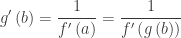Given that $f\left( 2 \right)=5\text{ and }{f}'\left( 2 \right)=3$ and g is the inverse of f, Find ${g}'\left( 5 \right)$ .

The solution is reasoned this way: (5, ?) is a point on g. The corresponding point on f is (?, 5) = (2, 5). The derivative of f at this point is 3, therefore the derivative at (5, 2) on g is ${g}'\left( 5 \right)=\tfrac{1}{3}$ .

Easy!

The Calculus of Inverses

Posted on November 12, 2012 by Lin McMullin

Today we will consider computing the derivative of the inverse of a function. This is pretty standard and is in all the textbooks.

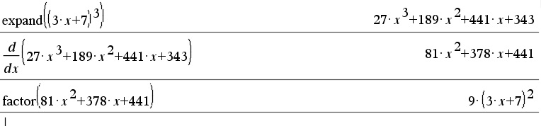
The usual suspects are the inverse trigonometric functions. So let’s start with $y={{\sin }^{-1}}\left( x \right)$ and then rewrite this as $x=\sin \left( y \right)$ . Differentiating this gives

$\displaystyle 1=\cos \left( y \right)\frac{dy}{dx}$
$\displaystyle \frac{dy}{dx}=\frac{1}{\cos \left( y \right)}$

Since we would like this in terms of x we can proceed two ways.

The denominator is the cosine of the number whose sine is x. So using the relationship

$\cos \left( y \right)=\sqrt{1-{{\sin }^{2}}\left( y \right)}=\sqrt{1-{{x}^{2}}}$

we find that

$\displaystyle \frac{dy}{dx}=\frac{1}{\sqrt{1-{{x}^{2}}}}$ .

That tends to be confusing so another method is to draw a right triangle with an acute angle of y and arrange the side so that

$\displaystyle \sin \left( y \right)=\frac{x}{1}=\frac{\text{opposite}}{\text{hypotenuse}}$

From this we can find all the trigonometric functions of y, specifically:

$\displaystyle \cos \left( y \right)=\frac{\text{adjacent}}{\text{hypotenuse}}-\frac{\sqrt{1-{{x}^{2}}}}{1}=\sqrt{1-{{x}^{2}}}$ and $\displaystyle \frac{dy}{dx}=\frac{1}{\sqrt{1-{{x}^{2}}}}$ .

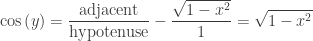
A second example: Find the derivative of $y={{\sec }^{-1}}\left( x \right)$ . The domain of this function is $\left| x \right|\ge 1$ and the range is $[0,\tfrac{\pi }{2})\cup (\tfrac{\pi }{2},\pi ]$ , the function is increasing on both parts of its domain; we will need to know this.

Proceeding as above we will find that

$\displaystyle \frac{dy}{dx}=\frac{1}{\sec \left( y \right)\tan \left( y \right)}$ .

Drawing a triangle as above and arranging the side so that sec(y) = x:

Then $\displaystyle \frac{dy}{dx}=\frac{1}{x\sqrt{1+{{x}^{2}}}}$ ,

But wait! It may be that x < 0, but ${{\sec }^{-1}}\left( x \right)$ is increasing and the derivative should always be positive. So, this needs to be adjusted to

$\displaystyle \frac{d}{dx}{{\sec }^{-1}}\left( x \right)=\frac{1}{\left| x \right|\sqrt{1+{{x}^{2}}}}$

These can be a bit tricky.

Next: the fifth and last posting in this series will look at the graphical and numerical aspects of the derivatives of a function and its inverse.

Real “Real-life” Graph Reading

Posted on October 29, 2012 by Lin McMullin

A few days ago, Paul Krugman wrote a blog about the job situation in the US. Evan J. Romer, a mathematics teacher from Conklin, NY, used it as the basis for a great exercise on reading the graph of the derivative, the subject of my last post. He posted the questions to the AP Calculus Learning Community. I liked them so much I have included them on my blog with Evan’s kind permission. The questions and solutions are here and on the Resources Tab above.

He used the graph below which shows the change in the number of non-farm jobs per month; in other words, the graph of a derivative of the number of people employed. The jagged graph is the data; the smooth graph is a model approximating the data.

The model is $\displaystyle C\left( t \right)=\frac{1000{{t}^{2}}}{{{t}^{2}}+40}-800$

From this Mr. Romer developed a series of questions very similar to AP questions. Don’t overlook the last note which discusses a “classic AP calculus mistake” made by the first person to reply to Krugman’s blog.

The first of Romer’s questions are integration questions, which you may not yet have gotten to with your class. Below is another graph of nearly the same data displayed as a bar graph. (Around February 2010 this was dubbed the “Bikini Graph” – if you look at the graph before that date you will see why.) It may be helpful in explaining the first of Romer’s questions to your class since each bar represents the change in the number of jobs for that month and leads into the concept of accumulation and the integral as the area between the graph and the axis. You can return to this when you introduce integration.

Thank You Evan.

Reading the Derivative’s Graph

Posted on October 26, 2012 by Lin McMullin

A very typical calculus problem is given the equation of a function, to find information about it (extreme values, concavity, increasing, decreasing, etc., etc.). This is usually done by computing and analyzing the first derivative and the second derivative. All the textbooks show how to do this with copious examples and exercises. I have nothing to add to that. One of the “tools” of this approach is to draw a number line and mark the information about the function and the derivative on it.

A very typical AP Calculus exam problem is given the graph of the derivative of a function, but not the equation of either the derivative or the function, to find all the same information about the function. For some reason, student find this difficult even though the two-dimensional graph of the derivative gives all the same information as the number line graph and, in fact, a lot more.

Looking at the graph of the derivative in the x,y-plane it is easy to very determine the important information. Here is a summary relating the features of the graph of the derivative with the graph of the function.

Feature	the function
${y}'$ > 0	is increasing
${y}'$ < 0	is decreasing
${y}'$ changes – to +	has a local minimum
${y}'$ changes + to –	has a local maximum
${y}'$ increasing	is concave up
${y}'$ decreasing	is concave down
${y}'$ extreme value	has a point of inflection

Here’s a typical graph of a derivative with the first derivative features marked.

Here is the same graph with the second derivative features marked.

The AP Calculus Exams also ask students to “Justify Your Answer.” The table above, with the columns switched does that. The justifications must be related to the given derivative, so a typical justification might read, “The function has a relative maximum at x = -2 because its derivative changes from positive to negative at x = -2.”

Conclusion	Justification
y is increasing	${y}'$ > 0
y is decreasing	${y}'$ < 0
y has a local minimum	${y}'$ changes – to +
y has a local maximum	${y}'$ changes + to –
y is concave up	${y}'$ increasing
y is concave down	${y}'$ decreasing
y has a point of inflection	${y}'$ extreme values

For notes on vertical asymptotes see

For notes on horizontal asymptotes see Other Asymptotes

Teaching Calculus

The pleasure lies not in discovering the truth, but in searching for it.

Tag Archives: derivative

At Just the Right Time

Experimenting with CAS – Chain Rule

The Derivatives of Exponential Functions

Inverses Graphically and Numerically

The Calculus of Inverses

Real “Real-life” Graph Reading

Reading the Derivative’s Graph

Share this:

Share this:

Share this:

Share this:

Share this:

Share this:

Share this: