A few weeks ago I covered some trigonometry classes for another teacher. They were studying polar and parametric graphs and the common curves limaçon, rose curves, cardioids, etc. I got to thinking about these curves. the next few posts will discuss what I learned. To help me see what was happening I made a Winplot animation. My “Roulette Generator” (RG) is a rather simple setup and turned out to be very well suited to study a variety of curves: cardioids, epicycloids, epitrochoids, hypochoids, and hypotrochoids to name a few. They are all examples of roulettes – curves generated by a point on a curve as it moves around anther curve. I considered only cases where both curves are circles. Calculus will make it appearance after the first few posts in this series. I hope you will find information here that will let you make a good project or investigation for calculus or precalculus students. The RG can be set to graph any number of situations as I will discuss. So here goes.
Roulettes – 1: Equations and the Roulette Generator.
In this post I will discuss the derivation of the parametric equations used to make the animations and some notes on how to use the RG. Later posts will discuss some of the various curves that result. I began with a simple cardioid.

Cardioid R = S = 1
A cardioid is defined as the locus of a point on a circle as it rolls without slipping around another circle with the same radius.
The setup described here will allow us to change the equations using sliders, for this and a number of related curves. The two circles with the same radii are shown in the figure below. The circle with center at C rolls counterclockwise around the circle with center at the origin, O. The point D traces the cardioid. The blue curve from F to D is the beginning of the cardioid.  The equations of the circles are: The circle centered at the origin with radius 1:

The moving circle with center at C and radius R:
 and
and
 .
.
The equation of the locus: In the figure above, the locus of the point marked D, as the moving circle rolls counterclockwise around the fixed circle, will be the path of the curves. A small portion of the curve is shown in blue running from F to D. In our investigations we will eventually want to place the moving point inside, on, or outside the moving circle. To do this we will use S as the distance from the center of the moving circle to the point we are watching. For the moment and for the simple cardioid, we will assume they are the same:  .
.
The ratio of the radius of the fixed circle to the radius of the moving circle is 1/R, and will be of interest. The ratio can be adjusted by changing R. We can, therefore, keep the fixed circle’s radius constant and equal to one.
We will use vectors to write the locus. Before writing the individual vectors consider first that the arc length on both circles is always the same for all the curves and combinations of their radii:
 .
.
Therefore,  . Then
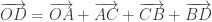
  Then the locus of D has the vector equation:


Notice that  is the complement of
  , so that
  and
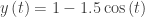
and  . The parametric equations of the path are


You may enter these equations on any graphing calculator by entering specific values of R and S. You will have to re-type them for each different curve. With the RG you can make the changes easily with sliders.
The roulette generators: I used Winplot a free graphing program I’ve used for years. Here are the links so you can download Winplot or Winplot for Macs. the Winplot file containing the generator is here: Winplot Roulette Generator. [Sorry, this is no longer available here and WordPress will not accept Winplot files for download. Please contact me at lnmcmullin@aol.com and I’ll send you a copy.] The Winplot equations are discussed here: Notes on the Roulette Generator.
A Geometer’s Sketchpad version may be downloaded Geometer’s Sketchpad Roulette Generator. You will need Geometer’s Sketchpad to run this on a computer or the “Sketch Explorer” app for iPads and other tablets. A big ‘Thanks” to Audrey Weeks who was kind enough to make this for us. Audrey is the author of the Algebra in Motion and Calculus in Motion software. Audrey is my “go to” person when I have math questions.
Other graphers with sliders such as Geogebra and TI-Nspire will probably work as well. For those who wish to adapt this to some other graphing program there are some syntax consideration to making the one circle roll around the other and showing the path as the circle rolls. If you make your own generator on one of these other platforms, please send it along and I’ll post it and give you credit.
Experiment with the R and S sliders. In the next several posts well will do this and learn about various other curves.
Next: Epicycloids
References:
Cardioids: http://en.wikipedia.org/wiki/Cardioid
Roulettes: http://en.wikipedia.org/wiki/Roulette_(curve)
Algebra in Motion
Calculus in Motion

 or the equivalent vector
  . The path is the curve traced by the parametric equations or the tips of the position vector. .
 . The vector sum of the components gives the direction of motion. Attached to the tip of the position vector this vector is tangent to the path pointing in the direction of motion.
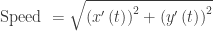 . (Notice that this is the same as the speed of a particle moving on the number line with one less parameter: On the number line
  .)
.) .
. , or even
  form. The pointed brackets seem to be the most popular right now, but all common notations are allowed and will be recognized by readers.
 . Notice that this is the integral of the speed (rate times time = distance).
 . See
. See 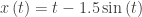
 .
. .
. .
. . This is a vector pointing in the direction of motion and whose length,
  , is the speed of the moving object.
 .
. .
.

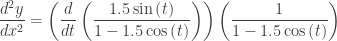
 is found by differentiating dy/dx, which is a function of t, implicitly with respect to x:
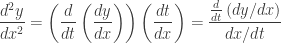


 indicating that the object will start by moving directly left. The green acceleration vector is
  pulling the velocity and therefore the object directly up. The second figure shows the vectors later in the first revolution. Note that the velocity vector is in the direction of motion and tangent to the path shown in blue.


