This is a good question that leads to other good questions, both mathematical and philosophical. A few days ago this question was posted on a private Facebook page for AP Calculus Readers. The problem and illustration were photographed from an un-cited textbook.
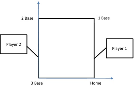
Player 1 runs to first base [from home plate] at a speed of 20 ft/s while player 2 runs from second base to third base a speed of 15 ft/s. Let s be the distance between the two players. How fast is s changing when player 1 is 30 feet from home plate and Player 2 is 60 feet from second base. [A figure was given showing that the distance between the bases is 90 feet.]

Some commenters indicated some possible inconsistencies in the question, such as assuming the Player 2 is on second base when Player 1 leaves home plate. In this case the numbers don’t make sense. So, someone suggested this must be a hit-and-run situation. To which someone else replied that with a lead of that much it’s really a stolen base situation. So, the first thing to be learned here is that even writing a simple problem like this you need to take some of the real aspects into consideration. But this doesn’t change the mathematical aspects of the problem.
One of the things I noticed before I attempted to work out the solution was that Player 2 is the same distance from third base as Player 1 is from home plate. I verbalized this as “players are directly across the field from each other.” I filed this away since it didn’t seem to matter much. Wrong!
Then I worked on the problem two ways. These are shown in the appendix at the end of this post. I discovered (twice) that s’ = 0; at the moment suggested in the question the distance is not changing.
Then it hit me. Doh! – I didn’t have to do all that. So, I posted this solution (which I now notice someone beat me to):
At the time described, the players are directly across the field from each other (90 feet apart). This is the closest they come. The distance between them has been decreasing and now starts to increase. So, at this instant s is not changing (s‘ = 0).
The Philosophical Question
Then the original poster asked for someone “to post [actual] work done in calculus” and “to see some related rates.” So, I posted some “calculus” and got to thinking – the philosophical question – isn’t my first answer calculus?
I think it is. It makes use of an important calculus concept, namely that as things change, at the minimum place, the derivative is zero. Furthermore, the justification (that the distance changes from decreasing to increasing at the minimum implies the derivative is zero) is included. * Why do you need variables?
Also, this solution is approached as an extreme value (max/min) problem rather than a related rate problem. This shows a nice connection between the two types of problems.
The Related (but not related rate) Good Question
So here is another calculus question with none of the numbers we’ve grown to expect:
Two cars travel on parallel roads. The roads are w feet apart. At what rate does the distance between the cars change when the cars are w feet apart?
Notice:
- That the cars could be travelling in the same or opposite directions.
- Their speeds are not given.
- You don’t know when or where they started; only that at some time they are opposite each other (w feet apart).
- In fact, they could start opposite each other and travel in the same direction at the same speed, remaining always w feet apart.
- One car could be standing still and the other just passes it.
But you can still answer the question.
(*Continuity and differentiability are given (or at least implied) in the original statement of the problem.)
Appendix
My first attempt was to set up a coordinate system with the origin at third base as shown below.

Then, taking the time indicated in the problem as t = 0, the position of Player 1 is (90, 30 + 20t) and the position of player 2 is (0, 30 – 15t). Then the distance between them is

and then

This is correct, but for some reason I was suspicious probably because zeros can hide things. So I re-stated this time taking t = 0 to be one second before the situation described in the problem. Now player 1’s position is (90, 10+20t) and player 2’s position is (0, 45-15t).


.
____________________________________________

 or the equivalent vector
  . The path is the curve traced by the parametric equations or the tips of the position vector. .
 . The vector sum of the components gives the direction of motion. Attached to the tip of the position vector this vector is tangent to the path pointing in the direction of motion.
 . (Notice that this is the same as the speed of a particle moving on the number line with one less parameter: On the number line
  .)
.) .
. , or even
  form. The pointed brackets seem to be the most popular right now, but all common notations are allowed and will be recognized by readers.
 . Notice that this is the integral of the speed (rate times time = distance).
 . See
. See 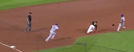
 .
. .
. .
. . This is a vector pointing in the direction of motion and whose length,
  , is the speed of the moving object.
 .
. .
.

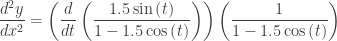
 is found by differentiating dy/dx, which is a function of t, implicitly with respect to x:
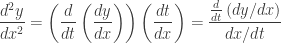


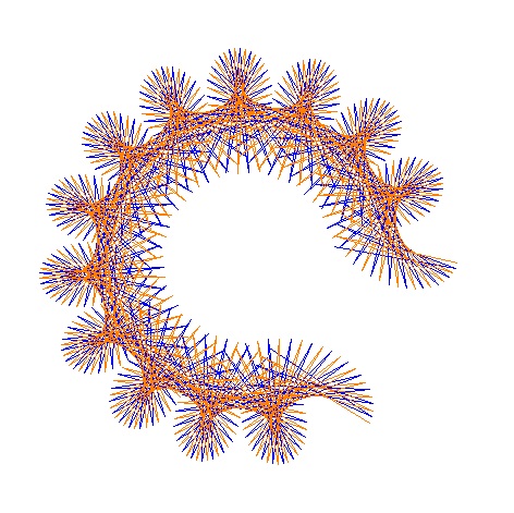
 indicating that the object will start by moving directly left. The green acceleration vector is
  pulling the velocity and therefore the object directly up. The second figure shows the vectors later in the first revolution. Note that the velocity vector is in the direction of motion and tangent to the path shown in blue.

 from the first. (From the previous posts: if
  then there are d dips, loops, or cusps in n full revolutions). Both graphs will have the same R value.


 , R = 0.00667 and slightly less than a full revolution. Make the image size (under the file tab) 12.3 x 12.3 (the units are cm.), or 465 x 465 pixels (type @ after the number to use pixels). Amazing!