Working Towards Riemann Sums

Posted on December 10, 2012 by Lin McMullin

In three previous posts (Nov 30, Dec 3 and Dec 5, 2012) we considered some examples leading up to integration and Riemann sums. Graphically all three can be seen as finding the area of the region between a graph and the x-axis over an interval. The next thing to do is to abstract that process and see if we can do this in general for any continuous function.

Most all of the textbooks do this in the same way and that’s probably what you should now lead your students through. Start with the simple basic case of a function that is positive, monotone, and continuous on an interval [a, b]. You wish to approximate the area of the region between the graph and the x-axis with vertical sides at x = a and x = b. (The actual minimum conditions are only that the function be bounded and continuous at all but a finite number of points. But that can wait.)

Follow the steps in your textbook.

The things you should emphasize first with numbers and then eventually with symbols are these.

The interval is divided into n sub-intervals each of equal length $\Delta x=\frac{b-a}{n}$ .
The x-coordinates of the endpoints are written in terms of a and $\Delta x$ . This is called a partition of the interval. The x-coordinates are $a={{x}_{0}}$ , ${{x}_{1}}=a+(1)\Delta x$ , ${{x}_{2}}=a+(2)\Delta x$ , ${{x}_{3}}=a+(3)\Delta x$ up to ${{x}_{n}}=a+(n)\Delta x=b$ .
Decide on a scheme to evaluate the function a one point in each of the sub-intervals defined by the partition. This is usually done at the left or right endpoint, but in fact may be anywhere in the sub-interval. The notation for this “any point” is $f\left( x_{i}^{*} \right)$ , which may be a little complicated. If you decide on using the right end then for the i^th sub-interval $[{{x}_{i-1}},{{x}_{i}}]$ the value is $f\left( {{x}_{i}} \right)$ , for the left side the value is $f\left( {{x}_{i-1}} \right)$ . This is the vertical distance between the graph and the x-axis.
Multiply this by the width of the sub-interval, this gives $f\left( {{x}_{i}} \right)\Delta x$ . Do this for each sub-interval and add the results to get your approximation. For the right side approximation this looks like $\sum\limits_{i=1}^{n}{f\left( {{x}_{i}} \right)\Delta x}$ .

Have your students compute this number for several functions with n in the 3 – 6 range. Your book will have plenty of examples. The idea is to learn and understand the procedure.

Some comments about each step above in case the kids ask. (Hope that they do.) Referring to the numbers above:

The sub-intervals do not have to be the same length. When we get to taking limits of the sum above, the actual requirement is that whatever way we partition the interval the largest sub-interval (called the norm of the partition) approaches zero in length as n increases. For actually doing the computation, equal length sub-intervals are easiest.
There will be a different $\Delta x$ for each interval: $\Delta {{x}_{i}}={{x}_{i}}-{{x}_{i-1}}$ .
You may pick any point in a sub-interval, and you do not even have to pick the same way in each sub-interval. For computation, the right side is usually the easiest, with the left side not far behind. For the theory involved, picking the largest and/or smallest value in each sub-interval is used. This value may not be at an endpoint.
Regardless of any of the above you will still multiply the function value by the width of the interval. The notation is more complicated. The sum is now written $\sum\limits_{i=1}^{n}{f\left( x_{i}^{*} \right)\left( {{x}_{i}}-{{x}_{i-1}} \right)}$

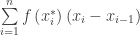
The important thing here is not the notation, but the process of partitioning the interval, calculating the function values multiplied by the width of the interval, and adding these products.

Under is a Long Way Down

Posted on December 7, 2012 by Lin McMullin

The development of the ideas and concepts related to definite integrals almost always begins with finding the area of a region between a graph in the first quadrant and the x-axis between two vertical lines. Everyone, including me in the past, refers to this as “finding the area under the curve.”

Under is a long way down. And while everyone understands what this means, I suggest that a better phrasing is “finding the area between the curve and the x-axis.” Here is why:

That is what you are doing.
You will soon be finding the area between the curve and the x-axis where the curve is below the x-axis. This often leads to something you may be tempted to call “negative area” and of course there is no such thing as a negative area, regardless of what you may find in some textbooks.

As with so many integration problems, the results is often a formula that obscures what is really going on – the Riemann sum whose value the integral gives. The first such formula is that the area is given by $\int_{a}^{b}{f\left( x \right)dx}$ . This is correct only if f (x) > 0. There is a natural confusion for beginning students between the facts that if f (x) < 0 the integral comes out negative, but the area is positive.

For all the applications of integration always emphasize the Riemann sum – not just the final formula. In the area problem with f (x) > 0 the integrand is the vertical length of the rectangles that make up the sum and this is the upper function’s value minus the lower function’s value, with the lower being the x-axis, y = 0. Then when f (x) < 0 the upper minus the lower is 0 – f (x) and the area is given by $\int_{a}^{b}{0-f\left( x \right)dx}=-\int_{a}^{b}{f\left( x \right)dx}$ which is positive as it should be. And students will immediately see that $\int_{a}^{b}{f\left( x \right)dx}$ is not automatically the area.

To help students see this you could start (very first problem) by helping them to find the area of the region between f (x) > 0 and the line y = 1 so they have to deal with the lower curve. Then consider another problem using the x-axis.

There is a fair amount of ground to cover between the first area between the curve and the x-axis problems with f (x) > 0 and other area problems. Teaching students how to set up those first Riemann sums, what a Riemann sum is, the definition of the definite integral and even the Fundamental Theorem of Calculus may all come between the first problem and when this distinction becomes important. Starting with the right words, “area between the graph and the x-axis”, will help in the long run.

Jobs, Jobs, Jobs

Posted on December 5, 2012 by Lin McMullin

Here is a problem similar to those in the last two posts; this one is based on a graph. The numbers are a little hard to read (sorry), but perhaps we do not need them. (If you want to do the numbers it is the second graph from the source which is more readable. There are other graphs of this type in the source, if you want some more.)

The discussion is aimed at relating the graph which is a derivative with the net change it describes. Thus, we are looking at determining increasing, decreasing, and relative extreme value from the graph and foreshadowing how this can be done using integration concepts especially accumulation.

Source: The Bureau of Labor Statistics

Some questions to discuss.

1. What are the units of this data, and what kind of units are they? (Thousands of jobs per month – a rate unit.)
2. Ask the students how they would find the total change in employment over the period given and discuss this with them. (Do not make them do the computation, just discuss how.)
3. Ask them to indicate on the graph when the total employment was the least and explain how they can tell from the graph (January 2010 – this is where the rate changes from negative to positive; this is the graph of a rate in thousands of jobs per month, therefore it is the derivative of jobs (employment)).
4. Ask how they could verify this by computing. What would they compute month-by-month? (The total number of jobs lost or gained from the beginning of the period – the accumulated change in jobs.)
5. During 2010 there is a local maximum in employment and another (local) minimum: when do they occur? How do you know without doing a computation?
6. What additional information do you need to tell how many people actually had jobs at any time during this period? (The total number employed at the beginning of 2008 – the initial condition.)

Flying to Integrationland

Posted on December 3, 2012 by Lin McMullin

Here is a problem similar to the one in the last post, but with foibles of its own.

The speed of an airplane in miles per hour is given at half-hour intervals in the table below. Approximately how far does the airplane travel in the three hours given in the table? How far is it from the airport?

Elapsed time (hours)	0	0.5	1	1.5	2	2.5	3
Speed (miles per hour)	375	390	400	390	385	350	345

In addition to just finding the estimates, compare this situation with the Pump Problem from the last post. Some points to consider

1. Answers between 1130 and 1145 miles are reasonable, if students proceed as they did with the Pump Problem. However, we cannot be sure since we do not know the speeds between the values recorded. In the Pump Problem we were told the pump was slowing down, so we could be sure the actual amount was between the values computed.
2. Based on the information in the table what is the low and high estimates of the total distance? What assumptions do you make for these estimates? (Low = 1117.5 miles, high = 1157.5 miles assuming the plane flew at the slowest (fastest) speed in the table for the entirety of each 1/2-hour interval.)
3. We also do not know where the plane started or which directions (plural) it was flying. So we have no way to tell how far it was from the airport (although we hope it gets to some airport eventually).
4. What are the units? If we graph this as we did in the Pump Problem the various rectangles have dimensions of (miles/hour) by hours, so the “area” is miles (a linear unit).

Next: Jobs, Jobs, Jobs

The Old Pump

Posted on November 30, 2012 by Lin McMullin

A tank is being filled with water using a pump that is old and slows down as it runs. The table below gives the rate at which the pump pumps at ten-minute intervals. If the tank initially has 570 gallons of water in it, approximately how much water is in the tank after 90 minutes?

Elapsed time (minutes)	0	10	20	30	40	50	60	70	80	90
Rate (gallons / minute)	42	40	38	35	35	32	28	20	19	10

And so begins integration.

Ask your students to do this problem alone. When they are ready (after a few minutes) collect their opinions. They will not all be the same (we hope, because there is more than one reasonable way to approximate the amount). Ask exactly how they got their answers and what assumptions they made. Be sure they always include units (gallons). Here are some points to make in your discussion – points that we hope the kids will make and you can just “underline.”

1. Answers between 3140 and 3460 gallons are reasonable. Other answers in that range are acceptable. They will not use terms like “left-sum”, “right sum” and “trapezoidal rule” because they do not know them yet, but their explanations should amount to the same thing. An answer of 3300 gallons may be popular; it is the average of the other two, but students may not have gotten it by averaging 3140 and 3460.
2. Ask if they think their estimate is too large or too small and why they think that.
3. Ask what they need to know to give a better approximation – more and shorter time intervals.
4. Assumptions: If they added 570 + 42(10) + 40(10) + … +19(10) they are assuming that the pump ran at each rate for the full ten minutes and then suddenly dropped to the next. Others will assume the rate dropped immediately and ran at the slower rate for the 10 minutes. Some students will assume the rate dropped evenly over each 10-minute interval and use the average of the rates at the ends of each interval (570 + 41(10) + 39(10) + … 14.5(10) = 3300).
5. What is the 570 gallons in the problem for? Well, of course to foreshadow the idea of an initial condition. Hopefully, someone will forget to include it and you can point it out.
6. With luck, someone will begin by graphing the data. If no one does, you should suggest it (as always) to help them see what they are doing graphically. They are figuring the “areas” of rectangles whose height is the rate in gallons/minute and whose width is the time in minutes. Thus the “area” is not really an area but a volume ((gal/min)(min) = gallons). In addition to unit analysis, graphing is important since you will soon be finding the area between the graph of a function and the x-axis in just this same manner.

Next post: Flying to Integrationland

Antidifferentiation

Posted on November 28, 2012 by Lin McMullin

Since a lot of classes start integration with antidifferentiation, I’ll discuss that first. If you decide to go with one of the other plans mentioned in my last post, then file this away for later.
____________

The key to finding antiderivatives is pattern recognition.

The simplest integrals are those that follow directly from derivatives such as. Students just need to recognize that the cosine is the derivative of the sine so $\int{\cos \left( x \right)dx}=\sin \left( x \right)+C$ . We wish they were all that simple.

Something like $\int{\tan \left( x \right){{\sec }^{2}}\left( x \right)dx}$ is more complicated. Is the integrand the derivative of $\tfrac{1}{2}{{\tan }^{2}}\left( x \right)$ or of $\tfrac{1}{2}{{\sec }^{2}}\left( x \right)$ ? The answer is yes.

The method called u-substitution helps in identifying the pattern of the integrand. To use this method identify some part of the integrand as a function which you call u and then calculate du and hope that the du is the rest of the integrand.

For $\int{\tan \left( x \right){{\sec }^{2}}\left( x \right)dx}$ you can try u = tan(x) and the du = sec²(x)dx and after making the substitutions:

$\int{\tan \left( x \right){{\sec }^{2}}\left( x \right)dx}=\int{udu}=\tfrac{1}{2}{{u}^{2}}=\tfrac{1}{2}{{\tan }^{2}}\left( x \right)+C$ .

On the other hand we could try u = sec(x) so that du = tan(x)sec(x)dx and

$\int{\tan \left( x \right){{\sec }^{2}}\left( x \right)dx}=\int{\sec (x)\left( \tan (x)\sec (x)dx \right)}$

$=\int{udu}=\tfrac{1}{2}{{u}^{2}}=\tfrac{1}{2}{{\sec }^{2}}\left( x \right)+C*$

(The + C* here not the same as the + C in the expression above: C* = C – ½.)

Either way students need to recognize that part of the integrand is the chain rule contribution to the derivative of the other part of the integrand. The usual three steps to acquire these pattern recognition skills are practice, practice, practice.

Another detail of u-substitution is handling missing constants. For example, $\int{\cos (2x)dx}$ .

Make the substitution u = 2x and then calculate du = 2dx so $dx=\tfrac{1}{2}du$ . Then making these substitutions

$\int{\cos (2x)dx}=\int{\cos \left( u \right)\left( \tfrac{1}{2}du \right)=}\tfrac{1}{2}\int{\cos \left( u \right)du=\tfrac{1}{2}\sin \left( u \right)}$ .

Then back-substituting: $\int{\cos (2x)dx}=\tfrac{1}{2}\sin \left( 2x \right)+C$ .

For simple u-substitutions like this I find it easier to think, and not write, u = 2x so du = 2dx and then write this multiplying by ½ outside the integral sign to account for the extra factor of 2.

$\int{\cos \left( 2x \right)dx=\tfrac{1}{2}\int{\cos \left( 2x \right)\left( 2dx \right)}}=\tfrac{1}{2}\sin \left( 2x \right)+C$ .

This idea only works with missing constants, since only constants can be moved in and out of integrands.

I explain the need for the constant to students by saying that the 2 appears (as if by magic) from the Chain Rule when you differentiate and therefore it must be present to disappear back into the Chain Rule when you antidifferentiate.

Point out to students that integration is very different than differentiation. Differentiation is pretty straightforward; you know what to do when you need to find a derivative. Antidifferentiation is more complicated since recognizing the form or pattern is necessary. The simpler looking integral $\int{\ln \left( x \right)}dx$ is really more difficult than $\int{\tfrac{\ln \left( x \right)}{x}dx}$ .

Finally, if you are teaching antiderivatives before beginning integration, when you get to definite integrals, you will have to remember to show students how to handle the limits of integration by using the same substitution.

For Advanced Placement AB calculus courses these (integrals that follow directly from derivatives and u-substitutions) are the only methods of integration tested. BC students also need to know integration by parts and partial fraction decomposition. I will discuss these later.

Absolutely

Posted on August 27, 2012 by Lin McMullin

Absolute Value

The majority of students learn about absolute value long before high school. That is, they learn a lot of wrong things about absolute value.

They learn that “the absolute value of a number is the number without its sign” or some such nonsense. All numbers, except zero have a sign! This sort of works with numbers, but becomes a problem when variables appear. True or false | x | = x? True or false | –x | = x? Most kids will say they are both true; in fact, as you know, they are both false.
They also learn that “the absolute value of a number is its distance from zero on the number line.” True and works for numbers, but what about variables?
They learn that “the absolute value of a number is the larger of the number and its opposite.” True again. How do you use it with variables?
They learn $\left| x \right|=\sqrt{{{x}^{2}}}$ which is correct, useful for order-of-operation practice, and useful in other ways later, But they still compute $\sqrt{{{\left( -3 \right)}^{2}}}=-3$ and $\sqrt{{{x}^{2}}}=x$ since the square and square “cancel each other out.”

So here is a good vertical team topic. Get to those teachers in elementary and middle school and be sure they are not doing any of the above. They should start with the correct definition in words:

The absolute value of a negative number is its opposite.
The absolute value of a positive number (or zero) number is the same number.

This works all the time and will continue to work all the time. Teaching anything else will eventually require unlearning what they are using, and unlearning is far more difficult than learning.

When they start using variables and reading symbols translated into English, then the definition becomes their first piecewise define function:

$\text{ If }x\ge 0,\text{ then }\ \left| x \right|=x;$ and if $x<0,\text{ then }\left| x \right|=-x$

$\left| x \right|=\left\{ \begin{matrix} x & \text{ if }x\ge 0 \\ -x & \text{ if }x<0 \\ \end{matrix} \right.$

When reading this definition be sure to say “the opposite of the number” not “negative x” which in this case is probably a positive number.

Give variations of the two True-False questions above on every quiz and test until everyone gets it right!

When you see absolute value bars and want to be rid of them the first question to ask is, “Is the argument positive or negative? “Any time there is an absolute value situation, this is the way to proceed.

And yes, this does show up on the AP Calculus exams. Consider $\int_{0}^{1}{\left| x-1 \right|dx}$ which appeared as a multiple-choice question a few years ago. Give it a try before reading on.

On the interval of integration, [0,1], $\left( x-1 \right)\le 0$ so $\left| x-1 \right|=-\left( x-1 \right)$

$\displaystyle \int_{0}^{1}{\left| x-1 \right|dx}=\int_{0}^{1}{-\left( x-1 \right)}dx=\left. -\tfrac{1}{2}{{x}^{2}}+x \right|_{0}^{1}=-\tfrac{1}{2}+1-0=\tfrac{1}{2}$

Now try $\displaystyle \int_{0}^{1}{\sqrt{{{x}^{2}}-2x+1}\,dx}$ , or did we do this one already?

Teaching Calculus

The pleasure lies not in discovering the truth, but in searching for it.

Category Archives: Integration Theory

Working Towards Riemann Sums

Under is a Long Way Down

Jobs, Jobs, Jobs

Flying to Integrationland

The Old Pump

Antidifferentiation

Absolutely

Absolute Value

Share this:

Share this:

Share this:

Share this:

Share this:

Share this:

Absolute Value

Share this: