Good Question 4: 2008 AB 10

Continuing my occasional series on Good Questions, today’s Good Question is a multiple-choice question from the 2008 AB Calculus exam, number 10. As an exam question it is only so-so, but it has a lot of potential for having a discussion of relative accuracy of Riemann sums in relation to the definite integral they approximate. The key to doing this is to look at the graph. The question relates the numerical and the graphical aspect of Riemann sums, two parts of the Rule of Four.

The question presented the graph of a function f, shown below and asked which of five answer choices has the least value. The choices were \displaystyle \int_{a}^{b}{f\left( x \right)}dx (which I will call I), the left Riemann sum approximation of the integral, L, the right Riemann sum approximation, R, the Midpoint Riemann sum approximation, M, and a Trapezoidal sum approximation, T. Each of the four approximations were to have 4 subintervals of equal length.

2008 AB 10

There are important things in the stem – namely that the graph is strictly decreasing and concave downward, and one unimportant thing – the number of subdivisions. As long as the graph is strictly monotonic and does not change concavity the number of subdivisions does not matter; the relative size of the five quantities will be the same. Therefore, to see which is least we can look at one subdivision covering the entire interval. That saves a lot of trouble and is worth discussing with your class. Usually, we let the number of subdivisions go off to infinity; here we go the other way.

Looking at a single interval from 1 to 3, it is easy to see by drawing or picturing the rectangle that the least Riemann sum will be R, the right Riemann sum.

So that answers the question, but there is a lot more you can do with the situation. The first that comes to mind is to have your students to put the five values in order from least to greatest. Stop here and try it for yourself.

R is the smallest and L is the largest. Since the top of a trapezoid between the endpoints of the function on the interval lies below the graph of the function, T is less than I.

So far we have R < T < I < L, but where does the midpoint Riemann sum fit in, and why?

2008 AB 10 b

Consider the figure above. C is the midpoint of segment AD.The area of the region between AD and the x-axis is the midpoint approximation. Segment BE is tangent to f(x) at C. Notice that \Delta ABC\cong \Delta DEC (Why?) and therefore, the area of the region between segment BE and the x-axis is the same as the area between segment AD and the x-axis. The midpoint approximation is the same as the area a trapezoid whose side is tangent to the graph at the midpoint of the interval and extending to the sides of the interval. So the midpoint approximation of the integral is greater than the integral. (The midpoint rectangle as the same area as the “midpoint trapezoid” and distinguishes it from the endpoint trapezoid).

Then R < T < I < M < L.

At least in this case.

In this case, the function was strictly decreasing and concave down. Have your class investigate other combinations of increasing and decreasing functions that are concave up and concave down. Ask your students, individually or in small groups, to investigate these different cases, and discover and justify that:

  1. There are four cases in all.
  2. The left sum is greatest, and the right sum is least when the function is strictly decreasing.
  3. The left sum is least, and the right sum is greatest when the function is strictly increasing.
  4. When the function is concave down, the endpoint trapezoid lies below the graph of the function and the midpoint trapezoid lies above the graph, therefore T < I < M.
  5. When the function is concave up, the endpoint trapezoid lies above the graph of the function and the midpoint trapezoid lies below the graph, therefore M < I < T.
  6. Consider cases where the function is below the x-axis.

Foreshadowing the FTC

This is an example to help prepare students to tackle the Fundamental Theorem of Calculus (FTC). Use it after the lesson on Riemann sums and the definition of the definite integral, but before the FTC derivation.

Consider the area, A, between the graph of f\left( x \right)=\cos \left( x \right) and the x-axis on the interval \left[ 0,\tfrac{\pi }{2} \right]. Set up a Riemann sum using the general partition:

 0={{x}_{0}}<{{x}_{1}}<{{x}_{2}}<{{x}_{3}}<\cdots <{{x}_{n-2}}<{{x}_{n-1}}<{{x}_{n}}=\tfrac{\pi }{2}

\displaystyle A=\int_{0}^{{\scriptstyle{}^{\pi }\!\!\diagup\!\!{}_{2}\;}}{\cos \left( x \right)dx}=\underset{\Delta x\to 0}{\mathop{\lim }}\,\sum\limits_{i=1}^{n}{\cos \left( {{c}_{i}} \right)\left( {{x}_{i}}-{{x}_{i-1}} \right)}

Since we can choose the value of {{c}_{i}} any way we want, let’s take the same intervals and use {{c}_{i}} the number guaranteed by the Mean Value Theorem for the function F\left( x \right)=\sin \left( x \right) on the each sub-interval interval.  That is, on each sub-interval at x={{c}_{i}}

\left. \frac{d}{dx}\sin \left( x \right) \right|_{x={{c}_{i}}}^{{}}=\cos \left( {{c}_{i}} \right)=\frac{\sin \left( {{x}_{i}} \right)-\sin \left( {{x}_{i-1}} \right)}{\left( {{x}_{i}}-{{x}_{i-1}} \right)}

Then, substituting into the Riemann sum above

\displaystyle A=\underset{\Delta x\to 0}{\mathop{\lim }}\,\sum\limits_{i=1}^{n}{\cos \left( {{c}_{i}} \right)\left( {{x}_{i}}-{{x}_{i-1}} \right)}=\underset{\Delta x\to 0}{\mathop{\lim }}\,\sum\limits_{i=1}^{n}{\frac{\sin \left( {{x}_{i}} \right)-\sin \left( {{x}_{i-1}} \right)}{\left( {{x}_{i}}-{{x}_{i-1}} \right)}\left( {{x}_{i}}-{{x}_{i-1}} \right)}

\displaystyle A=\underset{\Delta x\to 0}{\mathop{\lim }}\,\sum\limits_{i=1}^{n}{\left( \sin \left( {{x}_{i}} \right)-\sin \left( {{x}_{i-1}} \right) \right)}

Now writing out the terms we have a telescoping series:

\displaystyle A=\left( \sin \left( {{x}_{1}} \right)-\sin \left( {{x}_{0}} \right) \right)+\left( \sin \left( {{x}_{2}} \right)-\sin \left( {{x}_{1}} \right) \right)+\left( \sin \left( {{x}_{3}} \right)-\sin \left( {{x}_{2}} \right) \right)+

\displaystyle \cdots +\left( \sin \left( {{x}_{n-1}} \right)-\sin \left( {{x}_{n-2}} \right) \right)+\left( \sin \left( {{x}_{n}} \right)-\sin \left( {{x}_{n-1}} \right) \right)

\displaystyle A=\sin \left( {{x}_{n}} \right)-\sin \left( {{x}_{0}} \right)

\displaystyle A=\sin \left( \tfrac{\pi }{2} \right)-\sin \left( 0 \right)=1

As you can see, this is really just the derivation of the FTC applied to a particular function. Now the students should have a better idea of what’s going on when you solve the problem in general, i.e. when you prove the FTC.


Arbitrary Ranges

In my last post I discussed the idea that the ranges of the inverse trigonometric functions are chosen somewhat arbitrarily. For good reasons, the ranges always include the first quadrant and the adjoining quadrant (II or IV) where the function is negative. If possible, the range is also chosen to be continuous. Still the choices are arbitrary.

I discussed the range of the inverse tangent function in relation to the value of the improper integral \int_{0}^{\infty }{\frac{1}{1+{{x}^{2}}}dx}
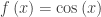
. I noted that if we used some other continuous range for the inverse tangent that the result of this or any other definite integral of this function gives the same value. Thus a range for the inverse tangent of \left( -\tfrac{\pi }{2},\tfrac{\pi }{2} \right),\left( \tfrac{\pi }{2},\tfrac{3\pi }{2} \right),\left( \tfrac{3\pi }{2},\tfrac{5\pi }{2} \right), etc. will give the same result.

For antiderivatives involving the inverse tangent or inverse cotangent this is true, but what about the other inverse trigonometric functions?

When evaluating the difference between two values as one does when evaluating a definite integral any range which results in a graph “parallel” to the graph over the commonly accepted range gives the same value.

However, for an integral requiring the inverse sine, if we use the range \left[ \tfrac{\pi }{2},\tfrac{3\pi }{2} \right],

\displaystyle \int_{0}^{1/2}{\frac{1}{\sqrt{1-{{x}^{2}}}}dx}=\left. {{\sin }^{-1}}\left( x \right) \right|_{0}^{1/2}

={{\sin }^{-1}}\left( \tfrac{1}{2} \right)-{{\sin }^{-1}}\left( 0 \right)=\tfrac{5\pi }{6}-\pi =-\tfrac{\pi }{6}

Indicating that a region above the x-axis has a negative area!

So \left[ \tfrac{\pi }{2},\tfrac{3\pi }{2} \right] is not a good choice. We could use other ranges for the inverse sine function but they would have to be such that they result in inverse sine graphs “parallel” to the usual graph. So we could use \left( \tfrac{3\pi }{2},\tfrac{5\pi }{2} \right) or \left( \tfrac{7\pi }{2},\tfrac{9\pi }{2} \right), but not \left( \tfrac{5\pi }{2},\tfrac{7\pi }{2} \right).

The same problem arises with the inverse cosine, the inverse secant, and the inverse cosecant.

It is best to stick with the commonly accepted ranges. Still, going off on tangents often helps sharpen a student’s understanding.


Improper Integrals and Proper Areas

A few years ago, on the old AP Calculus discussion group a teacher asked a question about this improper integral:

\displaystyle \int_{0}^{\infty }{\frac{1}{1+{{x}^{2}}}dx}=\underset{b\to \infty }{\mathop{\lim }}\,\int_{0}^{b}{\frac{1}{1+{{x}^{2}}}dx}

=\underset{b\to \infty }{\mathop{\lim }}\,\left. \left( {{\tan }^{-1}}\left( x \right) \right) \right|_{0}^{b}

=\underset{b\to \infty }{\mathop{\lim }}\,\left( {{\tan }^{-1}}\left( b \right)-{{\tan }^{-1}}\left( 0 \right) \right)=\frac{\pi }{2}  

His (quite perceptive) student pointed out that the range of the inverse tangent function is arbitrarily restricted to the open interval \left( -\tfrac{\pi }{2},\tfrac{\pi }{2} \right). The student asked if some other range would affect the answer to this problem. The short answer is no, the result is the same. For example, if range were restricted to say \left( \tfrac{5\pi }{2},\tfrac{7\pi }{2} \right), then in the computation above:

\underset{b\to \infty }{\mathop{\lim }}\,\left( {{\tan }^{-1}}\left( b \right)-{{\tan }^{-1}}\left( 0 \right) \right)=\tfrac{7\pi }{2}-3\pi =\tfrac{\pi }{2}

The value is the same. While that is pretty straightforward, there are other things going on here which may be enlightening. The original indefinite integral represents the area in the first quadrant between the graph of y=\frac{1}{1+{{x}^{2}}} and the x-axis. Let’s consider the function that gives the area between the y-axis and the vertical line at various values of x.

A \displaystyle\left( x \right)=\int_{0}^{x}{\frac{1}{1+{{t}^{2}}}}\ dt

Pretending for the moment that we don’t know the antiderivative, we can use a calculator to graph the area function. Improper integralOf course, we recognize this as the inverse tangent function, but what is more interesting is that whatever this function is, it seems to have a horizontal asymptote at y=\tfrac{\pi }{2}
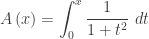
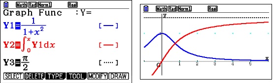
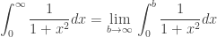
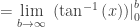
. The area is approaching a finite limit as x increases without bound.  The unbounded region has a finite area. The connection with improper integrals is obvious.

\displaystyle \underset{b\to \infty }{\mathop{\lim }}\,A\left( b \right)=\underset{b\to \infty }{\mathop{\lim }}\,\int_{0}^{b}{\frac{1}{1+{{x}^{2}}}dx=}\int_{0}^{\infty }{\frac{1}{1+{{x}^{2}}}dx}

Also, the improper integral is defined as the limit of the area function. This may give some insight as to why improper integrals are defined as they are.

Modified Tabular Integration

Several weeks ago, Dr. Qibo Jing, an AP teacher at Rancho Solano Preparatory School in Scottsdale, Arizona, posted a new way to approach tabular integration to the AP Calculus Community discussion group.  He calls this the Modified Tabular Method. The algorithm makes repeated integration by parts quicker and more streamlined than the usual method. The usual method is explained here.

Here is Dr. Jing’s method outlined and illustrated with this example \displaystyle I=\int{\left( {{x}^{3}}+7{{x}^{2}} \right)\cos \left( x \right)dx}

Step 1: Identify u and dv in the usual way and rewrite the given integral in terms of u={{x}^{3}}+7{{x}^{2}} and dv=\cos \left( x \right)=\tfrac{d}{dx}\sin \left( x \right).

\displaystyle I=\int{\left( {{x}^{3}}+7{{x}^{2}} \right)\cos \left( x \right)dx}=\int{\left( {{x}^{3}}+7{{x}^{2}} \right)\left( \tfrac{d}{dx}\left( \sin x \right) \right)}

Step 2: The first term of the antiderivative is the product of the two functions that appear in the revised integral:

\displaystyle I=\int{\left( {{x}^{3}}+7{{x}^{2}} \right)\left( \tfrac{d}{dx}\left( \sin x \right) \right)}=\left( {{x}^{3}}+7{{x}^{2}} \right)\sin \left( x \right)\cdots

Step 3: The remaining terms alternate sign. The next term has subtraction sign etc. The first factor of the next term is the derivative of the first factor of the current term. The second factor is the antiderivative of the second factor of the current term – differentiate the first factor; integrate the second factor.

\displaystyle I =\int{\left( {{x}^{3}}+7{{x}^{2}} \right)\left( \tfrac{d}{dx}\left( \sin x \right) \right)}=\left( {{x}^{3}}+7{{x}^{2}} \right)\sin \left( x \right)-\left( 3{{x}^{2}}+14x \right)\left( -\cos \left( x \right) \right)\cdots

Step 4: Alternate signs and repeat step 3 until the term becomes zero or until the original form appears (See next example). DO NOT simplify either factor until you are done as this may change later terms.

Modified A

The simplified result is

\displaystyle I=\left( {{x}^{3}}+7{{x}^{2}}-6x-14 \right)\sin \left( x \right)+\left( 3{{x}^{2}}+14x-6 \right)\cos \left( x \right)+C

Here is a second example.  In this example the original integral returns as the third term.

\displaystyle I=\int{{{e}^{x}}\sin \left( x \right)dx=\int{\sin \left( x \right)\left( \tfrac{d}{dx}{{e}^{x}}dx \right)}}

=\sin \left( x \right)\left( {{e}^{x}} \right)-\cos \left( x \right)\left( {{e}^{x}} \right)+\left( -\sin \left( x \right) \right)\left( {{e}^{x}} \right)

={{e}^{x}}\sin \left( x \right)-\cos \left( x \right)\left( {{e}^{x}} \right)-I

2I={{e}^{x}}\sin \left( x \right)-\cos \left( x \right)\left( {{e}^{x}} \right)

I=\tfrac{1}{2}\left( {{e}^{x}}\sin \left( x \right)-\cos \left( x \right)\left( {{e}^{x}} \right) \right)+C

This really is a simpler algorithm than the usual tabular method.

Variations on a Theme – 2

This is the second in an occasional series on adapting and expanding AP calculus exam questions. Variations on multiple-choice questions may make other multiple-choice questions, or, if you do not like making up all the “wrong” choices they can be changed to short answer questions for use in your class homework or test. Other variations make for good discussion questions.

 Today we will take a look at 2008 AB 10. This question gave the graph below and asked which of \displaystyle \int_{1}^{3}{f\left( x \right)dx}, a left, right, or midpoint Riemann sum approximation, or a trapezoidal sum approximation of the integral all with four subintervals of equal length has the least value.

Variations 2 pix 1

I’ll refer to these as I, L, R, M and T. The answer is R as a quick sketch will show.

In the discussion we will assume the curve does not change direction or concavity over the interval of integration. The answers to the questions in the variations are at the end of this post.

Variation 1: The question seems pretty easy so let’s beef it up a bit. How about asking the student to put I, L, R, M and T in order from smallest to largest? For a multiple-choice question answer choices are inequalities with all 5 sums in them.

The midpoint Riemann sum may be the most difficult to see. Here is the way to explain it. See the figure below.

Variations 2 pix 2

On each subinterval draw the horizontal segment at the function value at the midpoint of the interval. At this same point draw a tangent segment from one side of the interval to the other. This forms two congruent triangles with the horizontal segment and the edges of the interval.

Therefore, this midpoint trapezoid and the midpoint rectangle have the same area. Then because of the concavity, we see that in this case the midpoint Riemann sum, M, will be larger than the integral, I. With the same concavity the trapezoidal approximation will lie below the curve and therefore T < I < M. This will be true for any curve that is concave down. The opposite is true for a curve that is concave up: M < I < T. M and T are always on opposite sides of I. 

Variation 2: Change the number of subintervals, but keep the same number for each sum. Does this change anything?

Variation 3: Change the number of subintervals so that the sums over the same interval have a different number of subintervals. Does this change anything?

Variation 4: Change the shape of the curve to one of the other 4 shapes that a curve may have. How does this change the order of the sums?

Variation 5: Move the graph from above the ­x-axis to below. Does this change anything?

Variation 6: The reversal problem. Suppose that L < T < I < M < R; describe the shape of the curve. Other orders can be used as well. In fact this idea has appeared on an AP calculus exams. In 2003 AB 85 students were told that a trapezoidal sum over approximates and a right Riemann sum under approximates a certain integral. The question asked which of 5 graphs could be the graph of the function.

___________________

If you have other variations please click “Leave a Comment” to share them. If you have variations on a different question please share them as well.

___________________

Answers:

Variation 1: R < T < I < M < L

Variation 2: No. Since the order will be the same on each subinterval adding them will not change the order.

Variation 3: This makes a difference. In the first figure above, consider a trapezoidal sum with one subinterval compared to a right Riemann sum with many subintervals. The right Riemann sum will be very close to the integral with its rectangles ending above the trapezoidal segment between the endpoints. In this case T < R for the figure shown.

Variation 4: The left and right Riemann sums depend on whether the curve is decreasing or increasing. The Trapezoidal sum and the midpoint Riemann sum depend on the concavity. For example, an increasing concave up curve the order is L < M < I < T < R.

Variation 5: No. If the curve is entirely below the x-axis all the values will be negative, but all the results discussed in the other variations will be the same; the order will not change.

Variation 6: The curve is increasing and concave down.

Average Value of a Function

Today I want to consider a way of developing the expression for finding the average value of a function, f (x), on an interval [a, b].

Ask students how to find the average of a bunch of numbers and they will say, “add them up and divide by the number of numbers.” Then ask if they can average an infinite number of numbers. Most will say no since you cannot divide by infinity.

Well, what if the numbers were all the same?

Such as all the y-values of f (x) = 2 between x =1 and x = 5. Isn’t the average 2? So, apparently, you can sometimes average an infinite number of numbers.

Next suggest something like f (x) = x between x = 0 and x = 3. Since half the values are obviously above 1.5 and half below, can’t 1.5 be their average? Sketch this situation and draw the segment at y = 1.5 to help them see this.

Suggest another situation, say f (x) = 2 + sin(x) on the interval \left[ 0,2\pi \right] and some others. The average appears to be 2, again since half the values are above and half below 2.

When you draw the line that is the apparent average, lead the students to see that the rectangle formed by this line, the x-axis and the ends of the interval has the same area as between the function and the x-axis.

Continue with more difficult examples until someone hits on the idea of finding the “area” with an integral and then dividing the result by the width of the interval to find the height of the rectangle that is also the average value:

\displaystyle \overline{y}=\frac{\text{''area''}}{\text{length of interval}}=\frac{\int_{a}^{b}{f\left( x \right)dx}}{b-a}

Click here for an activity that you can use to develop this idea from scratch.

The next post: A fun application of average value – Most Triangles Are Obtuse.