
Volume by the method of “Cylindrical Shells”

Today I will show you how to visualize the cylindrical shells used in computing the volume using Winplot.
Winplot is a free program. Click here for Winplot and here for Winplot for Macs.
For the example I will use the same situation as in the last post. This was an AP question from 2006 AB1 / BC 1. In part (c) students were asked to find the volume of the solid figure formed when the region between the graphs of y = ln(x) and y = x – 2 is revolved around the y-axis. This can be done by the washer method, but some students use the method of cylindrical shells. We found that the graphs intersect at x = 0.15859 and x = 3.14619.
Begin as before by graphing the two functions and the vertical segment joining them.
- In Winplot open a 2D window, click on Equa > 1. Explicit and enter the first equation. Click the “lock interval” box and enter 0.159 for the “low x,” and 3.146 for the “high x,” choose a color and click “ok.”
- Repeat this for the second equation.
- Then return to Equa > Segment > (x,y) and enter the endpoints of the vertical segment joining the graphs: x1 = B, y1 = ln(B), x2 = B, and y2 = B – 2. Choose a color and click “ok.”
- Click Anim > individual > B to open a slider box for B. Type 0.159 and click “set L” and then type 3.146 and click “set R.” Use this slider to move the thin Riemann sum rectangle across the region.
Next draw the 3D graphs:
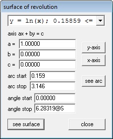
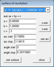
- Click One > Revolve Surface. The equations will appear in the drop-down box at the top of the window. Graphs are revolved one at a time. For the first graph click the “y-axis” button to put the correct values for a, b, and c in the boxes. In the “arc start” box type 0.159 and in the “arc stop” box type 3.146, the ends of the interval. In the “angle stop” box type 2pi@S. (S for surface.) See the figure below. Click “see surface.”
- Repeat this by selecting the second function from the drop-down box. Leave all the values the same and click enter. The two surfaces will be graphed in the same color as the corresponding functions in the 2D set up.
- Repeat this for the segment, but change the 2p@S in “arc stop” box to 2p@R. (R for Riemann rectangle.) Click “see surface.”
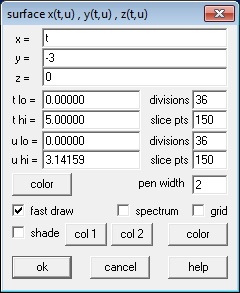
- You will need to make one adjustment at this point. In the 3D Inventory list choose the segment and click “edit.” In the box change “low t” to 0 and the “high t” to 1. See the next figure.

- In the 3D window, click Anim > Individual and open slider boxes for B, R, and S.
- In the B box enter 0.159 and click “set L” and enter 3.146 and click “set R.” These are the endpoints.
- In the S box make “set L” = -2pi. “Set R” should already be 2pi. Then type 0 and Enter.
- The R box should open with “set L” = 0 and “Set R” = 2pi. no changes are necessary.
- Move first the B slider, then the R slider, then the B slider again and finally the S slider to explore the situation.
- Type Ctrl+A to show the axes. Use the 4 arrow keys to move the figure around, and the page up and page down keys to zoom in and out.
That should do it.
In the video above you will see
- The Riemann rectangle moving in the plane using the B slider.
- The Riemann rectangle rotated around the y-axis using the R slider.
- The shell moving through the curves using the B slider again.
- The two curves rotated part way using the S slider.
- The shell moving through the solid using the B slider.
The next and last post in this series will be a question to see if you understand how the washer method and the cylindrical shell method work in a real situation.
Update:One of my favorite post is Difficult Problems and Why We Like Them from June 10, 2013. In it I mention a sculpture called Kryptos located at CIA headquarters in Langley, Virginia. The sculpture contains four enciphered messages. Only three of these have been deciphered since the sculpture was erected in 1990. The sculptor has offered a second clue to the fourth message. I’ve added links story and clues in the original post; see if you can decipher the fourth part.


 and
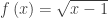
and  from x = 1 to x = 5.
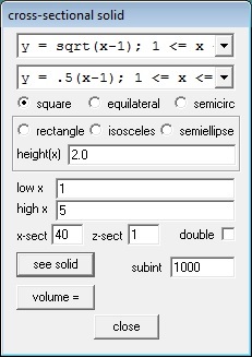
 Now let’s get fancy. Close the 3D window and return to the cross-section box shown above. Change the “high x” to 5@B (you may use any almost letter except x, y, or z). Then click “see solid.” Next, in the 3D Window click Anim > Individual > B. This will give you a slider. Slide the slider from 1 to 5 and you will see the solid grow and see the square cross-sections. (The video uses the “autocyc” button – use S to slow the animation, F to speed it up and Q to quit.)


 , which of the following values is the greatest?
 changes from positive to negative.”
  and the maximum value of
  ….” And then ask any of the questions above – some answers will be different, some will be the same. Discussing which will not change and why makes a worthwhile discussion.
 and ask the questions above. Again most of the answers will change.
  and ask the questions above. This time most of the answers will change.


