Unit 2 contains topics rates of change, difference quotients, and the definition of the derivative (CED – 2019 p. 51 – 66). These topics account for about 10 – 12% of questions on the AB exam and 4 – 7% of the BC questions.
Topics 2.1 – 2.4: Introducing and Defining the Derivative
Topic 2.1: Average and Instantaneous Rate of Change. The forward difference quotient is used to introduce the idea of rate of change over an interval and its limit as the length of the interval approaches zero is the instantaneous rate of change.
Topic 2.2: Defining the derivative and using derivative notation. The derivative is defined as the limit of the difference quotient from topic 1 and several new notations are introduced. The derivative is the slope of the tangent line at a point on the graph. Explain graphically, numerically, and analytically how the three representations relate to each other and the slope.
Topic 2.3 Estimating the derivative at a point. Using tables and technology to approximate derivatives is used in this topic. The two resources in the sidebar will be helpful here.
Topic 2.4: Differentiability and Continuity. An important theorem is that differentiability implies continuity – everywhere a function is differentiable it is continuous. Its converse is false – a function may be continuous at a point, but not differentiable there. A counterexample is the absolute value function, |x|, at x = 0.
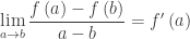
One way that the definition of derivative is tested on recent exams which bothers some students is to ask a limit like
 .
.
From the form of the limit students should realize this as the limit definition of the derivative. The h in the definition has been replaced by x. The function is tan(x) at the point where  . The limit is
  .
.
Topics 2.5 – 2.10: Differentiation Rules
The remaining topics in this chapter are the rules for calculating derivatives without using the definition. These rules should be memorized as students will be using them constantly. There will be additional rules in Unit 3 (Chain Rule, Implicit differentiation, higher order derivative) and for BC, Unit 9 (parametric and vector equations).
Topic 2.5: The Power Rule
Topic 2.6: Constant, sum, difference, and constant multiple rules
Topic 2.7: Derivatives of the cos(x), sin(x), ex, and ln(x). This is where you use the squeeze theorem.
Topic 2.8. The Product Rule
Topic 2.9: The Quotient Rule
Topic 2.10: Derivative of the other trigonometric functions
The rules can be tested directly by just asking for the derivative or its value at a point for a given function. Or they can be tested by requiring the students to use the rule of an general expression and then find the values from a table, or a graph. See 2019 AB 6(b)
The suggested number of 40 – 50 minute class periods is 13 – 14 for AB and 9 – 10 for BC. This includes time for testing etc. Topics 2.1, 2,2, and 2.3 kind of flow together, but are important enough that you should spend time on them so that students develop a good understanding of what a derivative is. Topics 2.5 thru 2.10 can be developed in 2 -3 days, but then time needs to be spent deciding which rule(s) to use and in practice using them. The sidebar resource in the CED on “Selecting Procedures for Derivative” may be helpful here.
Other post on these topics
DEFINITION OF THE DERIVATIVE
Local Linearity 1 The graphical manifestation of differentiability with pathological examples.
Local Linearity 2 Using local linearity to approximate the tangent line. A calculator exploration.
Discovering the Derivative A graphing calculator exploration
The Derivative 1 Definition of the derivative
The Derivative 2 Calculators and difference quotients
Difference Quotients 1
Difference Quotients II
Tangents and Slopes
Differentiability Implies Continuity
FINDING DERIVATIVES
Why Radians? Don’t do calculus without them
The Derivative Rules 1 Constants, sums and differences, powers.
The Derivative Rules 2 The Product rule
The Derivative Rules 3 The Quotient rule
Here are links to the full list of posts discussing the ten units in the 2019 Course and Exam Description.
2019 CED – Unit 1: Limits and Continuity
2019 CED – Unit 2: Differentiation: Definition and Fundamental Properties.
2019 CED – Unit 3: Differentiation: Composite , Implicit, and Inverse Functions
2019 CED – Unit 4 Contextual Applications of the Derivative Consider teaching Unit 5 before Unit 4
2019 – CED Unit 5 Analytical Applications of Differentiation Consider teaching Unit 5 before Unit 4
2019 – CED Unit 6 Integration and Accumulation of Change
2019 – CED Unit 7 Differential Equations Consider teaching after Unit 8
2019 – CED Unit 8 Applications of Integration Consider teaching after Unit 6, before Unit 7
2019 – CED Unit 9 Parametric Equations, Polar Coordinates, and Vector-Values Functions
2019 CED Unit 10 Infinite Sequences and Series


 has a (removable) discontinuity at x = 3, but no value there.
 there is no value of g(3) to use, and the derivative does not exist.
 . This function has a jump discontinuity at x = 1.
 and the limit will always be a number greater than 3 divided by zero and will not exist. Therefore, even though the slopes from both side of x =1 approach the same value, namely 2, the derivative does not exist at x = 1.
 factor squeezes the function to the origin; the added condition that
  makes the function continuous. Differentiating gives


 , so, substituting
  we have


 – Fermat unknowingly is using the derivative! After which he set it equal to 0 and solved to find the
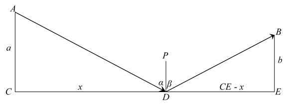
 and
and  are all perpendicular to
  the total distance is AD + DB. Therefore:
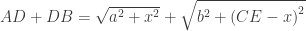


 and
and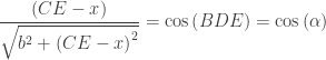
 QED.
QED.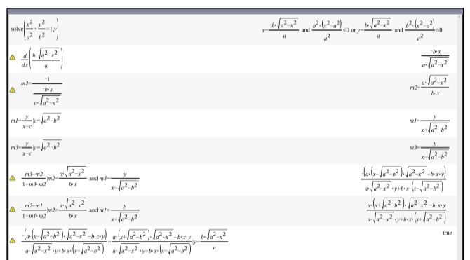
 with a > b > 0. Solving for y there are two equations, the second one is for the upper half that we will use below. The other for the lower half.
 and
and  .
. to avoid working with an undefined slope. The focus is at
  .
.