The Rate/Accumulation Question

Posted on March 1, 2013 by Lin McMullin

AP Type Questions 1

These questions are often in context with a lot of words describing a situation in which some things are changing. There are usually two rates given acting in opposite ways. Students are asked about the change that the rates produce over some time interval either separately or together.

The rates are often fairly complicated functions. If they are on the calculator allowed section, students should store them in the equation editor of their calculator and use their calculator to do any integration or differentiation that may be necessary.

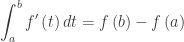
The integral of a rate of change is the net amount of change

$\displaystyle \int_{a}^{b}{{f}'\left( t \right)dt}=f\left( b \right)-f\left( a \right)$

over the time interval [a, b]. If the question asked for an amount, look around for a rate to integrate.

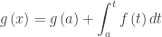
The final accumulated amount is the initial amount plus the accumulated change:

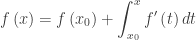
$\displaystyle f\left( x \right)=f\left( {{x}_{0}} \right)+\int_{{{x}_{0}}}^{x}{{f}'\left( t \right)}\,dt$ ,

where ${{x}_{0}}$ is the initial time, and $f\left( {{x}_{0}} \right)$ is the initial amount. Since this is one of the main interpretations of the definite integral the concept may come up in a variety of situations.

What students should be able to do:

Be ready to read and apply; often these problems contain a lot of writing which needs to be carefully read.
Recognize that rate = derivative.
Recognize a rate from the units given without the words “rate” or “derivative.”
Find the change in an amount by integrating the rate. The integral of a rate of change gives the amount of change (FTC):

$\displaystyle \int_{a}^{b}{{f}'\left( t \right)dt}=f\left( b \right)-f\left( a \right)$ .

Find the final amount by adding the initial amount to the amount found by integrating the rate. If $x={{x}_{0}}$ is the initial time, and $f\left( {{x}_{0}} \right)$ is the initial amount, then final accumulated amount is

$\displaystyle f\left( x \right)=f\left( {{x}_{0}} \right)+\int_{{{x}_{0}}}^{x}{{f}'\left( t \right)}\,dt$ ,

Understand the question. It is often not necessary to as much computation as it seems at first.
Use FTC to differentiate a function defined by an integral.
Explain the meaning of a derivative or its value in terms of the context of the problem.
Explain the meaning of a definite integral or its value in terms of the context of the problem. The explanation should contain (1) what it represents, (2) its units, and (3) how the limits of integration apply in context.
Store functions in their calculator recall them to do computations on their calculator.
If the rates are given in a table, be ready to approximate an integral using a Riemann sum or by trapezoids.
Do a max/min or increasing/decreasing analysis.

Shorter questions on this concept appear in the multiple-choice sections. As always, look over as many questions of this kind from past exams as you can find.

For some previous posts on this subject see January 21, 23, 2013

Interpreting Graphs

Posted on February 27, 2013 by Lin McMullin

AP Type Questions 1

The long name is “Here’s the graph of the derivative, tell me things about the function.”

Most often students are given the graph identified as the derivative of a function. There is no equation given and it is not expected that students will write the equation (although this may be possible); rather, students are expected to determine important features of the function directly from the graph of the derivative. They may be asked for the location of extreme values, intervals where the function is increasing or decreasing, concavity, etc. They may be asked for function values at points.

The graph may be given in context and student will be asked about that context. The graph may be identified as the velocity of a moving object and questions will be asked about the motion and position. (Motion problems will be discussed as a separate type in a later post.)

Less often the function’s graph may be given and students will be asked about its derivatives.

What students should be able to do:

Read information about the function from the graph of the derivative. This may be approached as a derivative techniques or antiderivative techniques.
Find where the function is increasing or decreasing.
Find and justify extreme values (1^st and 2^nd derivative tests, Closed interval test, aka. Candidates’ test).
Find and justify points of inflection.
Find slopes (second derivatives, acceleration) from the graph.
Write an equation of a tangent line.
Evaluate Riemann sums from geometry of the graph only.
FTC: Evaluate integral from the area of regions on the graph.
FTC: The function, g(x), maybe defined by an integral where the given graph is the graph of the integrand, f(t), so students should know that if, $\displaystyle g\left( x \right)=g\left( a \right)+\int_{a}^{t}{f\left( t \right)dt}$ then ${g}'\left( x \right)=f\left( x \right)$ and ${{g}'}'\left( x \right)={f}'\left( x \right)$ .

The ideas and concepts that can be tested with this type question are numerous. The type appears on the multiple-choice exams as well as the free-response. They have accounted for almost 25% of the points available on recent test. It is very important that students are familiar with all of the ins and outs of this situation.

As with other questions, the topics tested come from the entire year’s work, not just a single unit. In my opinion many textbooks do not do a good job with these topics.

Study past exams; look them over and see the different things that can be asked.

For some previous posts on this subject see October 15, 17, 19, 24, 26, 2012 January 25, 28, 2013

Introducing Power Series 1

Posted on February 8, 2013 by Lin McMullin

The next few posts will discuss a way to introduce Taylor and Maclaurin series to students. We will kind of sneak up on the idea without mentioning where we are going or using any special terms. In this post we will find a way of approximating a function with a polynomial of any degree we choose. In the next post we will look at the graph of these polynomials and finally suggest some questions for further thought.

Making Better Approximations

Students already know and have been working with the tangent line approximation of a function at a point (a, f(a)):

$f(x)\approx f\left( a \right)+{f}'\left( a \right)\left( x-a \right)$

ln(x):

For the function $f\left( x \right)=\ln \left( x \right)$ at the point (1, 0) ask your students to write the tangent line approximation: $y=0+(1)(x-1)$ .Point out that this line has the same value as ln(x) and its derivative as at (1, 0).

Then suggest that maybe having a polynomial that has the same value, first derivative and second derivative might be a better approximation. Suggest they start with $y=a+b\left( x-1 \right)+c{{\left( x-1 \right)}^{2}}$ and see if they can find values of a, b and c that will make this happen.

Since $f\left( 1 \right)=0,{f}'\left( 1 \right)=1\text{ and }{{f}'}'\left( x \right)=-1$ we can write

$y=a+b\left( x-1 \right)+c{{\left( x-1 \right)}^{2}};\quad y\left( 1 \right)=a+0+0=0;\quad a=0$

${y}'=b+2c\left( x-1 \right);\quad {y}'\left( 1 \right)=b+0=\tfrac{1}{1};\quad b=1$

${{y}'}'=2c;\quad {{y}'}'\left( 1 \right)=c=-\tfrac{1}{{{1}^{2}}}=-1;\quad c=-\tfrac{1}{2}$

$y=0+\left( x-1 \right)-\tfrac{1}{2}{{\left( x-1 \right)}^{2}}$

Then suggest they try a third degree polynomial starting with $y=a+b\left( x-1 \right)+c{{\left( x-1 \right)}^{2}}+d{{\left( x-1 \right)}^{3}}$ . Proceeding as above, all the numbers come out the same and we find that

$\ln \left( x \right)\approx 0+\left( x-1 \right)+\left( -\tfrac{1}{2} \right){{\left( x-1 \right)}^{2}}+\left( \tfrac{1}{3} \right){{\left( x-1 \right)}^{3}}$

Then go for a fourth- and fifth-degree polynomial until they discover the patterns. (The signs alternate, and the denominators are the factorial of the exponent.)

See if the class can write a general polynomial of degree N :

$\displaystyle \ln \left( x \right)\approx \sum\limits_{k=1}^{N}{\frac{{{\left( -1 \right)}^{k+1}}}{k}{{\left( x-1 \right)}^{k}}}$

sin(x):

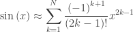
Then have the class repeat all this for a new function such as $f\left( x \right)=\sin \left( x \right)$ at the point (0, 0). This could be assigned as homework or group work. Ask them to do enough terms until they see the pattern. There will be patterns similar to ln(x ) and every other term (the even powers) will have a coefficient of zero.

$\sin \left( x \right)\approx x-\tfrac{1}{3!}{{x}^{3}}+\tfrac{1}{5!}{{x}^{5}}-\tfrac{1}{7!}{{x}^{7}}+\tfrac{1}{9!}{{x}^{9}}$

or in general the polynomial of degree N is

$\displaystyle \sin \left( x \right)\approx \sum\limits_{k=1}^{N}{\frac{{{\left( -1 \right)}^{k+1}}}{\left( 2k-1 \right)!}{{x}^{2k-1}}}$

How good is this approximation? Using only the first three terms of the polynomial above you will tell you that. Pretty close: correct to 5 decimal places. Using four terms gives correct to 7 decimal places when rounded.

Finally, see if they can generalize this idea to any function f at any point on the function $\left( {{x}_{0}},f\left( {{x}_{0}} \right) \right)$ . This time you will not have the various derivatives as numbers, rather they will be expressions like . Work through the powers one at a time to go from $y=a+b\left( x-{{x}_{0}} \right)+c{{\left( x-{{x}_{0}} \right)}^{2}}+d{{\left( x-{{x}_{0}} \right)}^{3}}+e{{\left( x-{{x}_{0}} \right)}^{4}}$

and so on, until you get to

$f\left( x \right)\approx f\left( {{x}_{0}} \right)+\frac{{f}'\left( {{x}_{0}} \right)}{1!}\left( x-{{x}_{0}} \right)+\frac{{{f}'}'\left( {{x}_{0}} \right)}{2!}{{\left( x-{{x}_{0}} \right)}^{2}}$

$\quad \quad \quad \quad \quad \quad \quad \quad \quad \quad \quad \quad \quad +\cdots +\frac{{{f}^{\left( N \right)}}\left( {{x}_{0}} \right)}{N!}{{\left( x-{{x}_{0}} \right)}^{N}}$

For example the third derivative computation would look like this:

${{{y}'}'}'=3\cdot 2\cdot 1d+4\cdot 3\cdot 2e\left( x-{{x}_{0}} \right)$

${{{y}'}'}'\left( {{x}_{0}} \right)=3\cdot 2\cdot 1d+4\cdot 3\cdot 2e(0)={{{f}'}'}'\left( {{x}_{0}} \right)$

$d=\frac{{{{f}'}'}'\left( {{x}_{0}} \right)}{3!}$

The computations here are perhaps a little different than what students have seen, so take your time doing this. Two or even three class days may be necessary.

Notice these things:

The first two terms are the tangent line approximation.
The various derivatives are numbers that must be calculated.
All the terms of any degree are the same as the terms of the previous degree with one additional term.

Next post in this series: Looking at all this graphically.

(Typos in an earlier version of this post have been corrected – LMc)

Logarithms

Posted on February 6, 2013 by Lin McMullin

Students first encounter logarithms in Algebra 2 or their last pre-calculus course. They are usually defined as exponents and their properties “proven” by reference to the corresponding properties of exponents. This is good enough at the time, but in calculus we are ready to define logarithms properly. The result is the definition in terms of a function defined by an integral.

In fact, the definition flows naturally from the properties of inverse functions (no pun intended, because the flow is quite natural). But is this a definition? Or a proof? The solution of certain differential equations discussed in my last post may be used to derive the logarithm function.

Let’s begin by pretending we know nothing about logarithms, and investigate the inverse of e^x. (See The Derivative of Exponential Functions)

This function e^x contains points of the form $\left( X,{{e}^{X}} \right)$ so its inverse will contain points of the form $\left( {{e}^{X}},X \right)$ , which, since we like the first coordinate of functions to be x, we may also call $\left( x,\ln \left( x \right) \right)$ , where ln(x) will be the name of the inverse of e^x. Remember, at the moment ln(x) is just a notation for the inverse of e^x, we do not know anything about logarithms (yet).

So $\left( {{e}^{X}},X \right)$ = $\left( x,\ln \left( x \right) \right)$ and $X\ne x$ . For example, (0, 1) is a point on e^X, so (1, 0) is a point on the ln(x) function, and so ln(1) = 0.

In a previous post we defined the number e and the function e^x in such a way that $\displaystyle \frac{d}{dx}{{e}^{x}}={{e}^{x}}$ . Now, at $\left( X,{{e}^{X}} \right)$ the derivative is e^X, so at the corresponding point on its inverse, $\left( {{e}^{X}},X \right)$ , the derivative is the reciprocal of the derivative of e^X which is $\frac{1}{{{e}^{X}}}=\frac{1}{x}$ . That is

$\displaystyle \frac{d}{dx}\ln \left( x \right)=\frac{1}{x}$

We can use this idea to define ln(x) as a function defined by an integral. Solving the differential equation by the method suggested in a recent post we get:

$\displaystyle \ln \left( x \right)=\ln \left( a \right)+\int_{a}^{x}{\frac{1}{t}dx}$

We can pick any positive number for a and a convenient one is the one we already found a = 1 where ln(1) = 0, so

$\displaystyle \ln \left( x \right)=\int_{1}^{x}{\frac{1}{t}dx},\quad x>0$

This then is the “official definition” of the natural logarithm function. The domain is x > 0 (the range of e^x) and the range is all real numbers (the domain of e^x).

Graphically, ln(x) is the area between the graph of $\displaystyle \frac{1}{t}$ and the t-axis between 1 and x. If $0<x<1$ , then $\ln \left( x \right)<0$ and if $x>1$ , $\ln \left( x \right)>0$ .

From this definition we can prove all the familiar properties of logarithms $\left( \ln \left( ab \right)=\ln \left( a \right)+\ln \left( b \right)\text{ etc}\text{.} \right)$ and show that this is a function of the kind we called “logarithm” all along. This is in all the textbooks so I will not go into this here.

One of these properties tells us that for $a>0\text{ and }a\ne 1$ , $\displaystyle {{\log }_{a}}\left( x \right)=\frac{\ln \left( x \right)}{\ln \left( a \right)}$ and since ln(a) is a constant

$\displaystyle {{\log }_{a}}\left( x \right)=\frac{1}{\ln \left( a \right)}\int_{1}^{x}{\frac{1}{t}dt}$

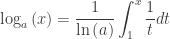
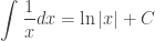
Finally, you will see this antiderivative formula: $\displaystyle \int_{{}}^{{}}{\frac{1}{x}dx=\ln \left| x \right|+C}$ . The absolute value sign is to remind you that the argument of the logarithm function must be positive, since in some situations x itself may be negative.

Revised slightly 8-28-2018

Inequalities

Posted on December 8, 2012 by Lin McMullin

This is an “extra” post on a technique that students are using a lot right now in graphing functions and working on optimization problems.

In analyzing a derivative to find critical points and then the intervals where the function increases and decreases you need to solve these inequalities. I’ve observed many students solving inequalities the hard way.

By that I mean they will pick a number in each interval between the critical points and then substitute it into the derivative and do a lot of arithmetic to determine whether the derivative is positive or negative. Arithmetic is not necessary, when all you really need is the sign of the derivative. The method I suggest is easier and involves no arithmetic and therefore precludes any arithmetic mistakes

A complete discussion of this idea with examples click here or look on my Resources page.

The Derivatives of Exponential Functions

Posted on November 21, 2012 by Lin McMullin

Our problem for today is to differentiate a^x with the (usual) restrictions that a is a positive number and not equal to 1. The reasoning here is very different from that for finding other derivatives and therefore I hope you and your students find it interesting.

The definition of derivative followed by a little algebra gives tells us that

$\displaystyle \frac{d}{dx}{{a}^{x}}=\underset{h\to 0}{\mathop{\lim }}\,\frac{{{a}^{x+h}}-{{a}^{x}}}{h}=\underset{h\to 0}{\mathop{\lim }}\,\frac{{{a}^{x}}{{a}^{h}}-{{a}^{x}}}{h}={{a}^{x}}\underset{h\to 0}{\mathop{\lim }}\,\frac{{{a}^{h}}-1}{h}$ .

Since the limit in the expression above is a number, we observe that the derivative of a^x is proportional to a^x. And also, each value of a gives a different constant. For example if a = 5 then the limit is approximately 1.609438, and so $\displaystyle \frac{d}{{dx}}{{5}^{x}}\approx \left( {1.609438} \right){{5}^{x}}$ .

I determined this by producing a table of values for the expression in the limit near x = 0. You can do the same using a good calculator, computer, or a spreadsheet.

h $\frac{{{5}^{h}}-1}{h}$

-0.00000030 1.60943752

-0.00000020 1.60943765

-0.00000010 1.60943778

0.00000000 undefined

0.00000010 1.60943804

0.00000020 1.60943817

0.00000030 1.60943830

That’s kind of messy and would require us to find this limit for whatever value of a we were using. It turns out that by finding the value of a for which the limit is 1 we can fix this problem. Your students can do this for themselves by changing the value of a in their table until they get the number that gives a limit of 1.

Okay, that’s going to take a while, but may be challenging. The answer turns out to be close to 2.718281828459045…. Below is the table for this number.

h $\frac{{{a}^{h}}-1}{h}$

-0.00000030 0.99999985

-0.00000020 0.99999990

-0.00000010 0.99999995

0.00000000 undefined

0.00000010 1.00000005

0.00000020 1.00000010

0.00000030 1.00000015

Okay, I cheated. The number is, of course, e. Thus,

$\displaystyle \frac{d}{{dx}}{{e}^{x}}={{e}^{x}}\left( {\underset{{h\to 0}}{\mathop{{\lim }}}\,\frac{{{{e}^{h}}-1}}{h}} \right)={{e}^{x}}(1)={{e}^{x}}$ .

The function e^x is its own derivative!

And from this we can find the derivatives of all the other exponential functions. First, we define a new function (well maybe not so new) which is the inverse of the function e^x called ln(x), the natural logarithm of x. (For more on this see Logarithms.) Then a = e^ln(a) and a^x = (e^ln(a))^x = e^(ln(a)x). Then using the Chain Rule, the derivative is

$\frac{d}{dx}{{a}^{x}}={{e}^{(\ln (a))x}}\ln (a)={{\left( {{e}^{\ln (a)}} \right)}^{x}}\ln (a)$

$\frac{d}{dx}{{a}^{x}}={{a}^{x}}\ln \left( a \right)$

Finally, going back to the first table above where a = 5, we find that the limit we found there 1.609438 = ln(5).

For a video on this topic click here.

Revised 8-28-2018, 6-2-2019

Speed

Posted on November 19, 2012 by Lin McMullin

Speed is the absolute value of velocity: speed = $\left| v\left( t \right) \right|$ .

This is the definition of speed, but hardly enough to be sure students know about speed and its relationship to velocity and acceleration.

Velocity is a vector quantity; that is, it has both a direction and a magnitude. The magnitude of velocity vector is the speed. Speed is a non-negative number and has no direction associated with it. Velocity has a magnitude and a direction. Speed has the same value and units as velocity; speed is a number.

The question that seems to trouble students the most is to determine whether the speed is increasing or decreasing. The short answer is

Speed is increasing when the velocity and acceleration have the same sign.

Speed is decreasing when the velocity and acceleration have different signs.

You should demonstrate this in some real context, such as driving a car (see below). Also, you can explain it graphically.

The figure below shows the graph of the velocity $v\left( t \right)$ (blue graph) of a particle moving on the interval $0\le t\le f$ . The red graph is $\left| v\left( t \right) \right|$ , the speed. The sections where $v\left( t \right)<0$ are reflected over the x-axis. (The graphs overlap on [b, d].) It is now quite east to see that the speed is increasing on the intervals [0,a], [b, c] and [d,e].

Another way of approaching the concept is this: the speed is the non-directed length of the vertical segment from the velocity’s graph to the t-axis. Picture the segment shown moving across the graph. When it is getting longer (either above or below the t-axis) the speed increases.

Thinking of the speed as the non-directed distance from the velocity to the axis makes answering the two questions below easy:

1. What are the values of t at which the speed obtains its (local) maximum values? Answer: x = a, c, and e.
2. When do the minimum speeds occur? What are they? Answer: the speed is zero at b and d

Students often benefit from a verbal explanation of all this. Picture a car moving along a road going forwards (in the positive direction) its velocity is positive.

If you step on the gas, acceleration pulls you in the direction you are moving and your speed increases. (v > 0, a > 0, speed increases)
Going too fast is not good, so you put on your brakes, you now accelerate in the opposite direction (decelerate?), but you are still moving forward, but slower. (v > 0, a < 0, speed decreases)
Finally, you stop. Then you shift into reverse and start moving backwards (negative velocity) and you push on the gas to accelerate in the negative direction, so your speed increases. (v < 0, a < 0, speed increases)
Then you put on the breaks (accelerate in the positive direction) and your speed decreases again. (v < 0, a > 0, speed decreases)

Here is an activity that will help your students discover this relationship. Give Part 1 to half the class and Part 2 to the other half. Part 3 (on the back of Part 1 and Part 2) is the same for both groups. – Added 12-19-17

Also see: A Note on Speed for the purely analytic approach.

Update: “A Note on Speed” added 4-21-2018

Teaching Calculus

The pleasure lies not in discovering the truth, but in searching for it.

Category Archives: Derivatives

The Rate/Accumulation Question

Interpreting Graphs

Introducing Power Series 1

Logarithms

Inequalities

The Derivatives of Exponential Functions

Speed

Share this:

Share this:

Share this:

Share this:

Share this:

Share this:

Share this: