A word before we look at one of my favorite AP exam questions, I put some of my presentations in a new page. Look under the “Resources” tab above, and you will see a new page named “Presentations.” There are PowerPoint slides and the accompanying handouts from some talks I’ve given in the last few years. I also use them in my workshops and AP Summer Institutes.
This continue a discussion of some of my favorite question and how to use them in class.You can find the others by entering “Good Question” in the search box on the right.
Today we look at one of my favorite AP exam questions. This one is from the 1995 BC exam; the question is also suitable for AB students. Even though it is 20 years old, it is still a good question. 1995 was the first year that graphing calculators were required on the AP Calculus exams.They were allowed, but not required for all 6 questions.
1995 BC 5
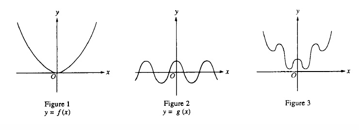
The question showed the three figures below and identified figure 1 as the graph of  and figure 2 as the graph of
  . The question then allowed as how one might think of the graph is figure 3 as the graph of
  , the sum of these two functions. Not that unreasonable an assumption, but apparently not correct.

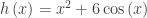
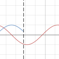
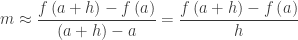
Part a: The students first were asked to sketch the graph of  in a window with [–6, 6] x [–6, 40] (given this way). A box with axes was printed in the answer booklet. This was a calculator required question and the result on a graphing calculator looks like this:

 .
.
The window is [-6,6] x [-6, 40]
Students were expected to copy this onto the answer page. Note that the graph exits the screen below the top corners and it does not go through the origin. Both these features had to be obvious on the student’s paper to earn credit.
Part b: The second part of the question instructed students to use the second derivative of to explain why the graph does not look like figure 3.


Students then had to observe that the second derivative was always positive (actually it is always greater than or equal to 1) and therefore the graph is concave up everywhere. Therefore, it cannot look like figure 3.
Part c: The last part of the question required students to prove (yes, “prove”) that the graph of  either had no points of inflection or infinitely many points of inflection, depending on the value of the constant k.
Successful student first calculated the second derivative:
Then considering the sign of the second derivative, if  ,
,  and there are no inflection points (the graph is always concave up). But, if
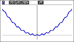
  , then since y” is periodic and changes sign, it does so infinitely many times and there are then infinitely many inflection points. See the figure below.

k = 8
Using this question as a class exercise
Notice how the question leads the student in the right direction. If they go along with the problem they are going in the right direction. In class, I would be inclined to make them work for it.
- First, I would ask the class if figure 3 is the correct graph of . I would let them, individually, in groups, or as a class suggest and defend an answer. I would not even suggest, but certainly not mind, if they used a graphing calculator.
- Once they determined the correct answer, I would ask them to justify (or prove) their conjecture. Again, no hints; let the class struggle until they got it. I may give them a hint along the lines of what does figure 3 have or do that the correct graph does not. (Answer: figure 3 changes concavity). Sooner or later someone should decide to check out the second derivative.
- Then I’d ask what could be the equation for a graph that does look like figure 3. You could give hints along the line of changing the coefficients of the terms of the second derivative. There are several ways to do this and all are worth considering.
- Changing the coefficient of the x2 term (to a proper fraction, say, 0.02) will do the trick. If that’s what they come up with fine – it’s correct.
- If you want to be picky, this causes the graph to go negative and figure 3 does not do that, but I ‘d let that go and ask if changing the coefficient of the cosine term in the second derivative can be done and if so how do you do that.
- This may be done by simply putting a number in front of the cosine term of the original function, say
 , but the results really do not look like figure 3,
- If necessary, give them the hint
1995 was the first year graphing calculators were required on the AP Calculus exams. They were allowed for all questions, but most questions had no place to use them. The parametric equation question on the same test, 1995 BC 1, was also a good question that made use of the graphing capability of calculators to investigate the relative motion of two particles in the plane. The AB Exam in 1995 only required students to copy one graph from their calculator.
Both BC questions were generally well received at the reading. I know I liked them. I was looking forward to more of the same in coming years.
I was disappointed.
There was an attempt the following year (1997 AB4/BC4), but since then nothing investigating families of functions (i.e. like these with a parameter that affects the shape of the graph) or anything similar has appeared on the exams. I can understand not wanting to award a lot of points for just copying the graph from your calculator onto the paper, but in a case like this where the graph leads to a rich investigation of a counterintuitive situation I could get over my reluctance.
But that’s just me.


 . This is a way of controlling the “a” slider and should always be multiplied by antiderivative. This is just a syntax trick to make the graph work and is not part of the antiderivative. When x is to the left of a, (x < a) the fraction is 1 and the graph will be seen; when x is to the right of a, (x > a) the expression is undefined, and nothing will graph. As you change “a” with the slider the graph of an antiderivative will be drawn.

 . A good second example is
  , and a third example to use is
  . Use simple functions, because you will want the students to see the answers without too much trouble.The procedure is the same for all.

 or
or 

 and, although it is easy enough to answer without, students were allowed to use their graphing calculator. A reasonable student probably looked at a graph of the function.
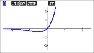
 and
and  . The students should not depend on the graph here. As
  ,
,  approaches zero and since the exponential function
  . In passing note that for x < 0 the function is negative and approaches zero from below. No work or explanation was required, but when teaching things like this be sure students know and can explain their answer without reference to their calculator graph. For the second limit, since both factors increase without bound
  If the student wrote
  , he received full credit.


 and if
  , therefore the absolute minimum is
  and occurs at
  , which may also be written as
  . (The decimals could also be used here.)
 where b was a non-zero number. The question required students to show that the absolute minimum value of all these functions was the same.
 and
and  .
.

 . The surface area including the top and bottom is given by
 , the surface area, S, can be expressed as
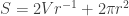
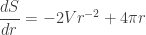
![\displaystyle r=\sqrt[3]{\frac{V}{2\pi }}](https://s0.wp.com/latex.php?latex=%5Cdisplaystyle+r%3D%5Csqrt%5B3%5D%7B%5Cfrac%7BV%7D%7B2%5Cpi+%7D%7D&bg=ffffff&fg=333333&s=0&c=20201002) and substituting into the expression above
and substituting into the expression above ![\displaystyle h=\sqrt[3]{\frac{4V}{\pi }}](https://s0.wp.com/latex.php?latex=%5Cdisplaystyle+h%3D%5Csqrt%5B3%5D%7B%5Cfrac%7B4V%7D%7B%5Cpi+%7D%7D&bg=ffffff&fg=333333&s=0&c=20201002) .
.![\displaystyle \frac{h}{r}=\sqrt[3]{\frac{\frac{4V}{\pi }}{\frac{V}{2\pi }}}=2](https://s0.wp.com/latex.php?latex=%5Cdisplaystyle+%5Cfrac%7Bh%7D%7Br%7D%3D%5Csqrt%5B3%5D%7B%5Cfrac%7B%5Cfrac%7B4V%7D%7B%5Cpi+%7D%7D%7B%5Cfrac%7BV%7D%7B2%5Cpi+%7D%7D%7D%3D2&bg=ffffff&fg=333333&s=0&c=20201002) , so
, so  . In the optimum can the height is equal to the diameter.
