From One Side or the Other.

Posted on November 1, 2016 by Lin McMullin

Recently, a reader wrote and suggested my post on continuity would be improved if I discussed one-sided continuity. This, along with one-sided differentiability, is today’s topic.

The definition of continuity requires that for a function to be continuous at a value x = a in its domain $\underset{x\to a}{\mathop{\lim }}\,f\left( x \right)=f\left( a \right)$ and that both values are finite. That is, the limit as you approach the point in question be equal to the value at that point. This limit is a two-sided limit meaning that the limit is the same as x approaches a from both sides. That definition is extended to open intervals, by requiring that for a function to be continuous on an open interval, that it is continuous at every point of the interval

How do you check every point? One way is to prove the limit in the definition in general for any point in the open interval. Another is to develop a list of theorems that allow you to do this. For example, f(x) = x can be shown to be continuous at every number. Then sums, differences, and products, of this function allows you to extend the property to polynomials and then other functions.

But what about a function that has a domain that is not the entire number line? Something like $f\left( x \right)=\sqrt{4-{{x}^{2}}},-2\le x\le 2$ . Here, $f\left( -2 \right)=f\left( 2 \right)=0$ ; the function is defined at the endpoints. A look at the graph shows a semi-circle that appears to contain the endpoints (–2, 0) and (2, 0). The function is continuous on the open interval (–2, 2) but cannot be continuous under the regular definition since the limit at the endpoints does not exist. The limit does not exist because the limit from the left at the left-endpoint, and the limit from the right at the right endpoint do not exist. What to do?

What is done is to require only that the one-sides limits from inside the domain exist. Here they do: $\underset{x\to -2+}{\mathop{\lim }}\,f\left( x \right)=0$ and the $\underset{x\to 2-}{\mathop{\lim }}\,f\left( x \right)=0$ and since the limits equal the values we say the function is continuous on the closed interval [–2, 2]. In general, when you say a function is continuous on a closed interval, you mean that the one-sided limits from inside the interval exist and equal the endpoint values.

You can determine that the limits exist by finding them as in the example above. Another way is to realize that if a < b < c < d and the function is continuous on the open (or closed) (a, d) then it is continuous on the closed interval [b c].

Why bother?

The reason we take this trouble is because for some reason the proof of the theorem under consideration requires that the endpoint value not only exist but hooks up with the function to make it continuous. Thus, the continuity on a closed interval is included in the hypotheses of theorem where this property is required. For example, the Intermediate Value Theorem would not work on a function that had no endpoints for $f\left( c \right)$ to be between. Also, the Mean Value Theorem requires you to find the slope between the endpoints, so the endpoint needs to be not only defined, but attached to the rest of the function.

One-sided differentiability

The definition of the derivative at a point also requires a two-sided limit to exist at the point. Most of the early theorems in calculus require only that the function be differentiable on an open interval.

Is it possible to define differentiability at the endpoint of an interval? Yes. It’s done in the same way by using a one-sided limit. If x = a is the left endpoint of an interval, then the derivative from the right at that point is defined as

$\displaystyle {f}'\left( a \right)=\underset{h\to 0+}{\mathop{\lim }}\,\frac{f\left( a+h \right)-f\left( a \right)}{h}$ .

By letting h approach 0 only from the right, you never consider values outside the interval. (At the right endpoint a similar definition is used with $h\to 0-$ ).

So why don’t we ever see one-sided derivatives? Because the theorems do not need them to prove their result. Hypotheses of theorems should be the minimum requirements needed, so if there is no need for the function to be differentiable at an endpoint, this is not listed in the hypotheses. This makes the hypothesis less restrictive and, therefore, covers more situations.

One theorem, beyond what is usually covered in beginning calculus, where endpoint differentiability is needed is Darboux’s Theorem. Darboux’s Theorem is sometime called the Intermediate Value Theorem for derivatives. It says that the derivative takes on all values between the derivatives at the endpoints, and thus needs the one-sided derivatives at the endpoints to exist. Interestingly, Darboux’s Theorem does not require the function to be continuous on the open interval between the endpoints.

Comparing the Graph of a Function and its Derivative

Posted on September 6, 2016 by Lin McMullin

The fourth in the Graphing Calculator / Technology series

Comparing the graph of a function and its derivative is instructive and necessary in beginning calculus. Today I will show you how you can do this first with Desmos a free online graphing program and then on a graphing calculator. Desmos does this a lot better than graphing calculators, because of the easy use of sliders. CAS calculators also have sliders but they are not as easy to use as Desmos.

Let’s get started. Instead of presenting you with a completed Desmos graph, I will show you how to make you own. One of the things I have found over the years is that it takes some mathematical knowledge to make good demonstration graph and that in itself if useful and instructive. Hopefully, you and your students will soon be able to make your own to show exactly what you want.

Open Desmos and sign into your account; if you don’t have one then register – its free and you can keep your results and even share them with others.

In the first entry line on the left, enter the equation of the function whose graph you want to explore. Call it f(x); that is enter f(x) = your function. Later you will be able to change this to other functions and investigate them, without changing anything else.

On the second line enter the symmetric difference quotient as

$\displaystyle s\left( x \right)=\frac{f\left( x+0.001 \right)-f\left( x-0.001 \right)}{2\left( 0.001 \right)}$

Instead of a variable h, as we did in our last post in this series, enter 0.001. This will graph the derivative without having to calculate the derivative. Of course, you could enter the derivative here if your class has learned how to calculate derivatives. If so, you will have to change this line each time you change the function.

In order to closely compare the function and its derivative, on the next line enter the equation of a vertical segment from a point on the function (a, f(a)) to a point on the derivative (a, s(a)). Desmos does not have a segment operation, but here is how you graph a segment. In general, a segment from (a, b) to (c, d) is entered as the parametric/vector function

$\left( a\cdot t+c\cdot \left( 1-t \right),b\cdot t+d\cdot \left( 1-t \right) \right),\ 0\le t\le 1$

The a, b, c, and d may be numbers or functions. Since our segment is vertical the first coordinate will have a = c and will reduce to a. Here’s what to enter on the third line:

$\left( a,f\left( a \right)\cdot t+s\left( a \right)\cdot \left( 1-t \right) \right)$

(Notice that there is no x in this expression; t is the variable. Also, the f(a) and s(a) may be interchanged.)

When you push enter, you will be prompted to add a slider for a: click to add the slider. A line will appear under the expression which will allow you to set the domain for t: click the endpoints and enter 0 on the left and 1 on the right, if necessary.

That’s it. You’re done. Use the slider to move around the graphs.

Using the graphs

Discuss with your class, or better yet divide them into groups and let them discuss, what they see. Since at this point they are probably new to this provide some hints such as “What happens on the graph of f when s is 0?” or “What is true on s when f is increasing?” or “What happens to the function at the extreme values of the derivative?” Prompt the students to look for increasing and decreasing, concavity, points of inflection, and extreme values. All the usual stuff. Work from the function to the derivative and from the derivative to the function.

Have your students formulate their results as (tentative) theorems. You actually want them to make some mistakes here, so you can help them improve their thinking and wording. For example, one result might be: If the function is increasing, then the derivative is positive. By changing the first function to an example like f(x) = x³ or f(x) = x + sin (x). Help them see that non-negative might be a better choice.

You might try giving different groups different functions and let them compare and contrast their results.

This is very much in line with MPACs 1, 2, 4, and 6.

You can do the same kind of thing with graphing calculators. That is, you can graph the function and its derivative or a difference quotient. The difference is that graphing calculators do not have sliders.

Extra feature: Desmos will graph a point if you enter the coordinates just like you write them: (a, b). The coordinates may be numbers or functions or a combination of both. Try adding two points to your graph one at each the end of the segment between the graphs that will move with the same slider.

f(x) = x + 2sin(x) and its derivative.

Seeing Difference Quotients

Posted on August 30, 2016 by Lin McMullin

Third in the graphing calculator series.

In working up to the definition of the derivative you probably mention difference quotients. They are

The forward difference quotient (FDQ): $\displaystyle \frac{f\left( x+h \right)-f\left( x \right)}{h}$

The backwards difference quotient (BDQ): $\displaystyle \frac{f\left( x \right)-f\left( x-h \right)}{h}$ , and

The symmetric difference quotient (SDQ): $\displaystyle \frac{f\left( x+h \right)-f\left( x-h \right)}{2h}$

Each of these is the slope of a (different) secant line and the limit of each as, if it exists, is the same and is the derivative of the function f at the point (x, f(x)). (We will assume h > 0 although this is not really necessary; if h < 0 the FDQ becomes the BDQ and vice versa.)

To see how this works you can graph a function and the three difference quotients on a graphing calculator. Here is how. Enter the function as the first function on your calculator and the difference quotients with it. Each of the difference quotients is defined in terms of Y1; this allows us to investigate the difference quotients of different functions by changing only Y1.

Now, on the home screen assign a value to h by typing [1] [STO] [alpha] [h]

Graph the result in a square window.

The look at the table screen. (Y1 has been turned off). Can you express Y2, Y3, and Y4 in term of x?

Then change h by storing a different value, say ½, to h and graph again. Then look at the table screen again. Can you express Y2, Y3, and Y4 in term of x?

Then graph again with h = -0.1

As you can see as h gets smaller (h 0), the three difference quotients are FDQ: 2x + h, the BDQ is 2x – h, and the SDQ is 2x. They converge to the same thing. The limit of each difference quotient as h approaches zero is twice the x coordinate of the point. If you’re not sure try a smaller value of h.

The function to which each of these converge is called the derivative of the original function (Y1). In the example the derivative of x² is 2x.

Now try another function say, Y1 = sin(x) and repeat the graphs and tables above. The tables will probably not be of much help, since the pattern is not familiar. The graph shows the function (dark blue) and only the SDQ (light blue), h = 0.1 Can you guess what the derivative might be?

I f you guessed cos(x) you are correct. The table shows the SDQ values as Y4, and the values of cos(x) as Y5. Pretty close! If you want to get closer try h = 0.001.

If you have a CAS calculators such as the TI-Nspire or the HP PRIME you can do this activity with sliders. Also you may try this with DESMOS. Click here or on the graph below. Some interesting functions to start with are cos(x) and | x |.

And by the way, the SDQ is what most graphing calculators use to calculate the derivative. It is called nDeriv on TI calculators.

Tangent Lines

Posted on August 23, 2016 by Lin McMullin

Second in the Graphing Calculator/Technology series

This graphing calculator activity is a way to introduce the idea if the slope of the tangent line as the limit of the slope of a secant line. In it, students will write the equation of a secant line through two very close points. They will then compare their results in several ways.

Begin by having the students graph a very simple curve such as y = x² in the standard window of their calculator. Then TRACE to a point. Students will go to different points, some to the left and some to the right of the origin. ZOOM IN several times on this point until their graph appears linear (discuss local linearity here). To be sure they are on the graph push TRACE again. The coordinates of their point will be at the bottom of the screen; call this point (a, b). Return to the home screen and store the values to A and B (click here for instructions on storing and recalling numbers).

Return to the graph and push TRACE again to be sure the cursor is on the graph. Move the TRACE cursor one or two pixels away from the first point in either direction. This new point is (c, d). Return to the home screen and store the coordinates to C and D.

Enter the equation of the line through the two points on the equation entry screen in terms of A, B, C, and D. Zoom Out several times until you have returned to the original window..

Exploration 1: Have students compare and contrast their graphs with several other students and discuss their observations. (Expected observations: the lines appear tangent at each students’ original point)

Exploration 2: Ask student to compute the slope of the line through their points, again using A, B, C, and D. Collect each student’s x-coordinate, A, and their slope and enter them in list is your calculator so that they can be projected.

Study the two lists and discuss the relation is any. (Expected observations: the slope is twice the x-coordinate.) Can you write an equation of these pairs? (Expected result: y = 2x)

Finally, plot the points on the calculator using a square window. Do the points seem to lie on the line y =2x?

Extensions:

Try the same activity with other functions such as y = (1/3)x³, y = x³, or y = x⁴. Anything more difficult will still result in a tangent line, but the numerical relationship between x and the slope will probably be too difficult to see. You may also consider y = sin(x) or y = cos(x). Again, the numerical work in Exploration 2, will be too difficult to see, but on graphing the points the result may be obvious. For y = sin(x), return to the list and add a column with the cosines of the x-values. Compare these with the slopes.

Tangents and Slopes

Posted on September 1, 2015 by Lin McMullin

Using the function to learn about its derivative.
In this post we will look at a way of helping students discover the numerical and graphical properties of the derivative and how they can be determined from the graph of the function. These ideas can be used very early, when you are first relating the function and its derivative. (In my next post we will look at the problem the other way around – using the derivative to find out about the function.)
Click on the graph below. This will take you to a graph I posted on the Desmos website (Desmos.com). This is a free and really easy to use grapher, which you and your students can use. If you sign up for your own account, you can make and save graphs for your class or use some of those that are built-in (click on the three horizontal bars at the upper left of the screen). Your students may do this as well. There are also Desmos apps for smart phones and tablets.

When you click on the graph a file called “function => derivative” should open. This is what you should see:
On the left is a list of equations. Those with a colored circle to its left are turned on; click the circle to toggle the graphs on and off. Here’s what they do:

f(x) is the equation of the function we will start with. Later you may change this to whatever function you are investigating. You will not have to change any of the others when you change the function. This one should be turned on.
g(x) is the derivative of f(x). Leave this turned off.
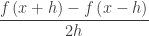
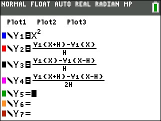
h(x) is a special function. The expression at the end, $\frac{\sqrt{a-x}}{\sqrt{a-x}}$ , is what makes the slider work. This is a syntax trick and not part of the derivative. If x is to the right of a (i.e. x < a) the expression is equal to one and the derivative will graph. If x is to the right of a, (i.e. a < x) then the expression is undefined, and nothing will graph. Initially, turned off.
k(x) is the graph of a segment tangent to f at x = a. Click on the equation if you want to see how the segment is drawn by restricting the domain of x. Initially, turned on.
The next equation, x = a, is the equation of the dashed vertical line. This is included so that, later, we can see precisely how points on the graph are located above one another. Initially, turned off.
(a, f(a)) is the point of tangency. Initially, turned on.
The last box is the slider for the variable a. Its domain is shown at the ends. This may be changed by clicking on one end or clicking on the “gear” icon at the top of the list.

The icons at the top right of the graph let you zoom in and out or set the viewing window. You may click on the wrench icon and make other adjustments. “Projector Mode” makes the graph thicker and may help students see better when you project the graph.
Okay, you are now Desmos experts! Really, it’s that easy. The “?” at the top right has a few more instructions and you can download the user’s guide, a brief 13 pages.

Investigating the derivative
Do this before proving all the associated theorems. Let the class discover the relations between the graph of the function and its derivative. Prove them, or explain why they are so, later. You may want to spread all this over several days, perhaps dealing with where the function is increasing or decreasing and extreme values the first day and working with concavity the second.
1. Begin with just f(x), k(x), and the point (a, f(a)) turned on (click the circle to the left of the equation to toggle graphs on and off). Use the slider to move the tangent segment along the graph.
Draw the class’s attention to important things but let them formulate the observations in words. Ask your class a series of questions about what they see. Things like:

When the function is increasing, is the slope of the tangent segment positive or negative? When the function is decreasing, is the slope of the tangent segment positive or negative? Why?
What happens with the derivative when the function changes from increasing to decreasing or vice versa?
Notice that sometimes the tangent segment lies above the function and sometimes below. What does the function look like when the tangent is above (below)?
In the box for the slider delete the number and type a = 0; this moves the slider to the origin. Can you see what its slope is here? You can type in other numbers such as pi/6, or pi/2 and read the slope there. (If the slider disappears when you do this, type in a = 0 and it will come back.)
If you can project on a white board or are using a Smartboard, mark the points (a, slope at a) and see if you can graph the derivative.

2. Next turn on h(x) and x = a. Move the slider.

What are you seeing? As you move the slider the dashed vertical line moves to show you where you are. The graph of the derivative is drawn to the left of the dashed line.
Once again question the class about what they observe. Notice such things as on intervals where the function increases, the derivative is greater than or equal to zero, etc. Review all the things you discovered in part 1. Remember often students don’t associate things such as “the derivative is negative” with the “graph of the derivative lies below the x-axis.“
How does the concavity relate to the graph of the derivative?

3. Now change the starting function to something else.

First, just add a constant to f(x). If you really want to get fancy type f(x) = sin(x) + b. A slider for b will appear. Discuss why this transformation does not change the graph of the derivative one bit.
Some good examples are f(x) = cos(x), f(x) = x+2sin(x), a third- or fourth-degree polynomial (find a good example in your textbook and see below). Repeat all of steps 1 and 2 above.

Give the students a new function and see if they can sketch the (approximate) graph of the derivative themselves.

For further exploration click the graph below. This is similar to the first one; however, the function is a fourth degree polynomial with variable coefficients. Use the various sliders at the bottom to adjust the graph to an interesting shape. Make p = 0 to graph a cubic and make both p and q zero to graph a parabola. (This might make a good lesson in an advanced math or Algebra 2 class.)

A disclaimer: A function and its derivative should not be graphed on the same axes, because the two have different units. Nevertheless, I have done it here, and it is commonly done everywhere to compare the graphs of a function and its derivatives so that the important features of the two can be lined up and compared easily.

Discovering the Derivative

Posted on August 18, 2015 by Lin McMullin

Discovering the Derivative with a Graphing Calculator

This is an outline of how to introduce the idea that the slope of the line tangent to a graph can be found, or at least approximated, by finding the slope of a line through two very close points in the graph. It is a set of graphing calculator activities that will use graphs and numbers to lead to the symbolic form of the derivative.

You may work through the activities with your class (which is what I would do) or you could write and distribute them and let your class do them a laboratory exercise. Before starting students should know how to use their calculator to graph, to trace to points on the graph, and how to save and recall the coordinates from the graph to variables on the home screen using the graphing calculator’s store feature.

I suggest you work through these three times (or more) using different functions. I will work with $y={{x}^{2}}$ . A good second example is $y={{x}^{3}}$ , and a third example to use is $y=\sin \left( x \right)$ . Use simple functions, because you will want the students to see the answers without too much trouble.The procedure is the same for all.

Part 1:

Begin by asking students to enter $y={{x}^{2}}$ in their calculator asY1 and graph it in a standard, square window. (Do not use the decimal window as “nice” decimals are not necessary or helpful.)
Figure 1
Next, have them trace over to different points on the graph (some should go left and others to the right); they should all end up at different points. Then have them zoom-in 6 or 8 times until the graph looks linear. (This is local linearity – functions that are differentiable are locally linear.)
Then push TRACE to be sure the cursor is on the graph. The coordinates of the point are on the bottom of the screen. Go to the HOME screen and save the two values as a and b. Think of this first point as (a, b).
Return to the graph screen and push TRACE. This should return the cursor to the first point. (If not, close is okay.) Then click to the right or to left once, or twice at most, to move to a nearby point on the graph. Return to the home screen and save the new values to c and d for the second point (c, d).
On the home screen use a, b, c, and d to write the slope of the line through the two points. See figure 1. (Go around the room as they are doing this and make sure students are getting this – their slope should be approximately twice a or c.)
Return to the equation screen and enter the equation of the line through the two points asY2. (See figure 2). Graph this equation with the parabola.
Figure 2
Have the students record their values of a, b, c, d and m on paper (three decimal places will be enough) and also write a description of what they see on the graph and why they think this is so. (This is in case they lose the numbers on their calculator when they do another graph and also because you will need them later in the next part of the exploration.)

Repeat the same steps separately with the other two functions and record the results in the same way. Write their numbers and observations. Discuss the observations with the class.

Of course, the lines should look tangent to the graphs, but since they contain two points of the graph, they cannot actually be tangent.
Discuss how a line can be tangent to a graph. How is this different from a tangent to a circle?
Ask what could be done to make their line even closer to being tangent. (Use points closer together.)

Part 2:

Now you have homework to do. Collect the student’s data and combine it into a list with columns for a, c, and m. The points do not have to be in order. Leave any “wrong” points for discussion; if there are none, you might want to make one up and include it. Do this for each of the three sets of data. Make a copy for each student. Enter the numbers for a and m as lists in your emulator and make a dot-plot of the points (a, m) = (a, slope at x = a).

Return the lists of points to the students and ask them to study the list and see if they can see any obvious relationship between the numbers on each line. Answers for y = x² should be the m is approximately twice either a or c; or maybe some will see that m is approximately a + c. Answers for y = x³ will be less obvious (three times the square of a). Answers for y = sin(x) will not be obvious at all.
Using the emulator, separately for each of the three sets of data, make a dot-plot of the numbers (use a square window). Ask the student to discuss what they see. See if they can find an equation of the graph of the dot-plots. Now the equation of the data set for sin(x) should be obvious. Plot their guesses on top of the points and see how close they come.

Part 3:

Now guide the class through the symbolic explanation of what they did. Ask them to explain and write in symbols specifically what they did. The idea here is for you, the teacher, to ask lots of leading questions until the class decides on the best answer.

Call the first point (a, f(a)). Let h = “a little bit.” then the second is the point (a plus a little bit, f(a plus a little bit)) or (a + h, f(a + h)). Recall that h may have been negative for some students so the second point may actually be to the left of the first. Then help them come up with

$\displaystyle m\approx \frac{f\left( a+h \right)-f\left( a \right)}{\left( a+h \right)-a}=\frac{f\left( a+h \right)-f\left( a \right)}{h}$

Or they may prefer

$\displaystyle m\approx \frac{f\left( a \right)-f\left( c \right)}{a-c}$

Ask how this could be made “less approximate” and more actually equal. (Answer: smaller and smaller value of h.) Ask them to find the value of h = a – c for their points. How small are they? How can you make them really small? (Find a limit.)
Notice that h cannot be zero in these expressions. Keep hinting until someone comes up with the idea of finding

$\displaystyle \underset{h\to 0}{\mathop{\lim }}\,\frac{f\left( a+h \right)-f\left( a \right)}{h}$ or $\displaystyle \underset{a\to c}{\mathop{\lim }}\,\frac{f\left( a \right)-f\left( c \right)}{a-c}$

Next have the students calculate the limits below by actually doing the algebra. (They will not be able to handle the sin(x) at this point so save that for later.)

$\displaystyle \underset{h\to 0}{\mathop{\lim }}\,\frac{{{\left( x+h \right)}^{2}}-{{\left( x \right)}^{2}}}{h}\text{ and }\underset{h\to 0}{\mathop{\lim }}\,\frac{{{\left( x+h \right)}^{3}}-{{\left( x \right)}^{3}}}{h}$

Compare the answers here with the earlier work and guesses, and discuss.

… And now you are ready to define the limits as the f ’(a) derivative of f at x = a.

Teaching Calculus

The pleasure lies not in discovering the truth, but in searching for it.

Category Archives: Derivative Theory

From One Side or the Other.

Comparing the Graph of a Function and its Derivative

Using the graphs

Seeing Difference Quotients

Tangent Lines

Tangents and Slopes

Discovering the Derivative

Discovering the Derivative with a Graphing Calculator

Share this:

Share this:

Using the graphs

Share this:

Share this:

Share this:

Share this:

Discovering the Derivative with a Graphing Calculator

Share this: