What’s the “Best” Error Bound?

Posted on January 28, 2020 by Lin McMullin

A know a lot of people like mathematics because there is only one answer, everything is exact. Alas, that’s not really the case. Numbers written as non-terminating decimals are not “exact;” they must be rounded or truncated somewhere. Even things like $\sqrt{7},\pi ,$ and 5/17 may look “exact,” but if you ever had to measure something to those values, you’re back to using decimal approximations.

There are many situations in mathematics where it is necessary to find and use approximations. Two if these that are usually considered in introductory calculus courses are approximating the value of a definite integral using the Trapezoidal Rule and Simpson’s Rule and approximating the value of a function using a Taylor or Maclaurin polynomial.

If you are using an approximation, you need and want to know how good it is; how much it differs from the actual (exact) value. Any good approximation technique comes with a way to do that. The Trapezoidal Rule and Simpson’s Rule both come with expressions for determining how close to the actual value they are. (Trapezoidal approximations, as opposed to the Trapezoidal Rule and Simpson’s Rule per se, are tested on the AP Calculus Exams. The error is not tested.) The error approximation using a Taylor or Maclaurin polynomial is tested on the exams.

The error is defined as the absolute value of the difference between the approximated value and the exact value. Since, if you know the exact value, there is no reason to approximate, finding the exact error is not practical. (And if you could find the exact error, you could use it to find the exact value.) What you can determine is a bound on the error; a way to say that the approximation is at most this far from the actual value. The BC Calculus exams test two ways of doing this, the Alternating Series Error Bound (ASEB) and the Lagrange Error Bound (LEB). These two techniques are discussed in my previous post, Error Bounds. The expressions used below are discussed there.

Examining Some Error Bounds

We will look at an example and the various ways of computing an error bound. The example, which seems to come up this time every year, is to use the third-degree Maclaurin polynomial for sin(x) to approximate sin(0.1).

Using technology to twelve decimal places sin(0.1) = 0.099833416647

The Maclaurin (2n – 1)^th-degree polynomial for sin(x) is

$\displaystyle x-\frac{1}{{3!}}{{x}^{3}}+\frac{1}{{5!}}{{x}^{5}}-+\cdots \frac{1}{{\left( {2n-1} \right)!}}{{x}^{{2n-1}}}$

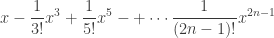
So, using the third degree polynomial the approximation is

$\sin \left( {0.1} \right)\approx 0.1-\frac{1}{6}{{\left( {0.1} \right)}^{3}}=0.099833333333...$

The error to 12 decimal places is the difference between the approximation and the 12 place value. The error is:

$\displaystyle 0.00000008331349=8.331349\times {{10}^{{-8}}}=Error$

Using the Alternating Series Error Bound:

Since the series meets the hypotheses for the ASEB (alternating, decreasing in absolute value, and the limit of the n^th term is zero), the error is less than the first omitted term. Here that is

$\displaystyle \frac{1}{{5!}}{{\left( {0.1} \right)}^{5}}\approx 0.0000000833333\approx 8.33333\times {{10}^{-8}}={{B}_{1}}$

The actual error is less than B₁ as promised.

Using the Legrange Error Bound:

For the Lagrange Error Bound we must make a few choices. Nevertheless, each choice gives an error bound larger than the actual error, as it should.

For the third-degree Maclaurin polynomial, the LEB is given by

$\displaystyle \left| {\frac{{\max {{f}^{{(4)}}}\left( z \right)}}{{4!}}{{{(0.1)}}^{4}}} \right|$ for some number z between 0 and 0.1.

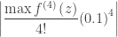
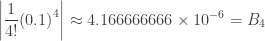
The fourth derivative of sin(x) is sin(x) and its maximum absolute value between 0 and 0.1 is |sin(0.1)|. So, the error bound is

However, since we’re approximating sin(0.1) we really shouldn’t use it. In a different example, we probably won’t know it.

What to do?

The answer is to replace it with something larger. One choice is to use 0.1 since 0.1 > sin(0.1). This gives

$\displaystyle \left| {\frac{{0.1}}{{4!}}{{{(0.1)}}^{4}}} \right|\approx 4.166666666\times {{10}^{{-7}}}={{B}_{3}}$

The usual choice for sine and cosine situations is to replace the maximum of the derivative factor with 1 which is the largest value of the sine or cosine.

$\displaystyle \left| {\frac{1}{{4!}}{{{(0.1)}}^{4}}} \right|\approx 4.166666666\times {{10}^{{-6}}}={{B}_{4}}$

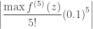
Since the 4^th degree term is zero, the third-degree Maclaurin Polynomial is equal to the fourth-degree Maclaurin Polynomial. Therefore, we may use the fifth derivative in the error bound expression, $\displaystyle \left| {\frac{{\max {{f}^{{(5)}}}\left( z \right)}}{{5!}}{{{(0.1)}}^{5}}} \right|$ to calculate the error bound. The 5^th derivative of the sin(x) is cos(x) and its maximum value in the range is cos(0) =1.

$\displaystyle \left| {\frac{{\max {{f}^{{(4)}}}\left( z \right)}}{{4!}}{{{(0.1)}}^{4}}} \right|$ for some number z between 0 and 0.1.

I could go on ….

Since B₁, B₂, B₃, B₄, and B₅are all greater than the error, which should we use? Or should we use something else? Which is the “best”?

The error is what the error is. Fooling around with the error bound won’t change that. The error bound only assures you your approximation is, or is not, good enough for what you need it for. If you need more accuracy, you must use more terms, not fiddle with the error bound.

Good Question 17

Posted on January 21, 2020 by Lin McMullin

A common question in (older?) textbooks is to give students a function or relation and have them graph it without technology (because in the old days technology was not available). Students had to find all the appropriate information without hints or further direction: they were supposed to know what to do and do it.

AP exam questions, for legitimate and understandable reasons, do not ask for as complete an analysis. Rather, they ask students to find specific information about the function or its graph (extreme values, points of inflection, etc.). For the same legitimate and understandable reason many of the features are not considered; the other concepts are tested on different questions.

I think that the full-analysis-from-scratch approach, while not appropriate for an AP exam question, has its merits. The big difference is that students need to be creative in their investigation; not just focus on a few items pointed to by the question.

With that in mind, let’s consider the following question asked three ways.

A very general form

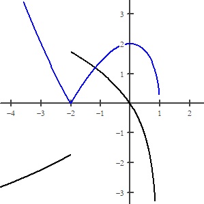
Consider the relation ${{x}^{3}}+3{{x}^{2}}+{{y}^{2}}=4$ . Discuss the graph of the relation giving reasons for your conclusions. Include a brief mention of any unproductive paths you followed and what you learned from them.

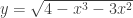
A more directed investigation

Consider the relation ${{x}^{3}}+3{{x}^{2}}+{{y}^{2}}=4$ . Find its extreme values and any asymptotes, and vertical tangents (if any). Discuss in detail the appearance of the graph near x = –2 and discuss the slopes in that area. Explain how you arrived at your results.

Closer to an AP style form. The function here is the top half of the function above.

Consider the function $y=\sqrt{{4-{{x}^{3}}-3{{x}^{2}}}}$ .

(a) Find the local maximum and minimum values of the function. Justify your answer.

(b) Where does the function had a vertical asymptote? Justify your answer.

(c) Find $\underset{{x\to -2-}}{\mathop{{\lim }}}\,\frac{{dy}}{{dx}}$ and $\underset{{x\to -2+}}{\mathop{{\lim }}}\,\frac{{dy}}{{dx}}$ . What does this say about the graph?

The real question is can you ask it the first way?

Here is my solution to the first form; this will also give the answers to the other forms. After the solution, I’ll discuss some ideas on how to score such a solution.

Solution

The graph of the relation ${{x}^{3}}+3{{x}^{2}}+{{y}^{2}}=4$ . is shown in figure 1.

Figure 1

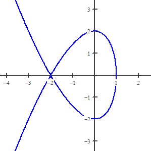
The domain of the function is $x\le 1$ . Values greater than 1 will make the left side of the equation greater than 4 regardless of the value of y. The range of the relation is all real numbers.

The function is symmetric to the x-axis since substituting (–y) for y will give the same expression. The equation of the top half is $y=\sqrt{{4-{{x}^{3}}-3{{x}^{2}}}}$ and the lower half is $y=-\sqrt{{4-{{x}^{3}}-3{{x}^{2}}}}$

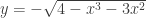
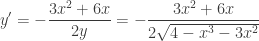
The derivative for the top half is $\displaystyle {y}'=-\frac{{3{{x}^{2}}+6x}}{{2y}}=-\frac{{3{{x}^{2}}+6x}}{{2\sqrt{{4-{{x}^{3}}-{3{x}^{2}}}}}}$ by implicit differentiation or by differentiating the equation for the top half.

$y'\left( x \right)$ does not exist at x = 1 specifically, $\displaystyle \underset{{x\to 1-}}{\mathop{{\lim }}}\,{y}'\left( x \right)=-\infty$ . Therefore, the line x = 1 is a vertical tangent. By symmetry for the lower part of the graph $\displaystyle \underset{{x\to 1-}}{\mathop{{\lim }}}\,{y}'\left( x \right)=+\infty$ . And x = 1 is its vertical asymptote as well. The slope of the original relation changes from positive to negative at x = 1 by going not through zero but from $-\infty$ to $+\infty$ .

${y}'\left( x \right)=0$ when x = 0 and when x = –2. At (0, 2) the derivative changes from positive to negative; this is a local maximum point by the first derivative test. The lower half has a local minimum point at (0, –2) by symmetry.

At (–2, 0) the derivative is an indeterminate form of the type 0/0.

False step: At first, I thought this meant that the two sides were tangent to the line x = –2 making the point (–2, 0) on the top half a cusp. I tried to see if this was true by graphing in a very narrow window. This did not show anything: the graph looked on zooming in, like an absolute value graph. It turned out that an absolute value was involved.

I then made a table of values for the derivative near the point and found that the values appeared to be approaching a number near –1.7 from the left and near +1.7 from the right. I started thinking maybe $\displaystyle \sqrt{3}$ .

Then I changed the constants to parameters and played with the sliders on Desmos (here). With a slight change in the constants the graph appeared to have a nice rounded local minimum near x= –2. Other values showed two separate pieces with vertical tangents near x= –2. This confused me even more.

Next, I did what I should have done earlier: I graphed the top half and its derivative (figure 2):

Figure 2. The top half in blue and its derivative in black.

The derivative has a finite jump discontinuity at x = –2. I remembered seeing this kind of thing before and thought it involved an absolute value of some kind. Still confused, I decided to investigate the derivative further (which I also should have done sooner).

The derivative at x = –2 is an indeterminate form of the 0/0 type. This means that by substituting you get an expression that really doesn’t help; you may still evaluate the limit (remember derivatives are limits) by other methods. Factoring the derivative (using synthetic division on the radicand) gives

$\displaystyle {y}'\left( x \right)=-\frac{{3x\left( {x+2} \right)}}{{2\sqrt{{{{{\left( {x+2} \right)}}^{2}}\left( {1-x} \right)}}}}=-\frac{{3x\left( {x+2} \right)}}{{2\sqrt{{{{{\left( {x+2} \right)}}^{2}}}}\sqrt{{1-x}}}}=-\frac{{3x}}{{\sqrt{{1-x}}}}\frac{{x+2}}{{\left| {x+2} \right|}}$

And now we see that

$\displaystyle \underset{{x\to -2-}}{\mathop{{\lim }}}\,\frac{{-3x}}{{2\sqrt{{1-x}}}}\cdot \frac{{x+2}}{{\left| {x+2} \right|}}=-\sqrt{3}$ and $\displaystyle \underset{{x\to -2+}}{\mathop{{\lim }}}\,\frac{{-3x}}{{2\sqrt{{1-x}}}}\cdot \frac{{x+2}}{{\left| {x+2} \right|}}=\sqrt{3}$

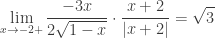
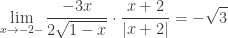
This agrees with the derivative’s graph. The top graph (and bottom’s by symmetry) comes to an arrow-like point (sometimes called a node) at (–2, 0). The slope on the left approaches $-\sqrt{3}$ and on the right approaches $+\sqrt{3}$ .

______________________

I admit I’ve had a few more years of experience with this sort of thing that a first-year calculus student. I expect this would be difficult for most students who have never seen a question like this, so working up to it with simpler questions is how to start.

In grading this sort of question, you need to consider:

If the student found and justified all the pertinent features of the graph. If they missed something, what they included may still be pretty good. For example, I would not expect a student to the use the word “node,” so omitting it should not be held against them and using it may call for praise.
The things they (and I) may have overlooked or things they considered that were unnecessary or even wrong.
Their overall approach. This last may be the most important part. Including their missteps and unproductive paths is important and should, I think, receive credit. After all, they did not know the path would be unproductive until they followed it a way. Hopefully, they made some missteps and learned something from them. That’s what investigating something in math entails.

I would be happy to hear if you tried this or something similar and so would the other readers of this blog. Please use the “Comment” button below to share your thoughts.

2019 CED Unit 10: Infinite Sequences and Series

Posted on January 14, 2020 by Lin McMullin

Unit 10 covers sequences and series. These are BC only topics (CED – 2019 p. 177 – 197). These topics account for about 17 – 18% of questions on the BC exam.

Topics 10.1 – 10.2

Timing

The suggested time for Unit 9 is about 17 – 18 BC classes of 40 – 50-minutes, this includes time for testing etc.

Previous posts on these topics :

Introducing Power Series 1

2019 CED Unit 9: Parametric Equations, Polar Coordinates, and Vector-Valued Functions

Posted on January 7, 2020 by Lin McMullin

Unit 9 includes all the topics listed in the title. These are BC only topics (CED – 2019 p. 163 – 176). These topics account for about 11 – 12% of questions on the BC exam.

Comments on Prerequisites: In BC Calculus the work with parametric, vector, and polar equations is somewhat limited. I always hoped that students had studied these topics in detail in their precalculus classes and had more precalculus knowledge and experience with them than is required for the BC exam. This will help them in calculus, so see that they are included in your precalculus classes.

Topics 9.1 – 9.3 Parametric Equations

Topic 9.1: Defining and Differentiation Parametric Equations. Finding dy/dx in terms of dy/dt and dx/dt

Topic 9.2: Second Derivatives of Parametric Equations. Finding the second derivative. See Implicit Differentiation of Parametric Equations this discusses the second derivative.

Topic 9.3: Finding Arc Lengths of Curves Given by Parametric Equations.

Topics 9.4 – 9.6 Vector-Valued Functions and Motion in the plane

Topic 9.4 : Defining and Differentiating Vector-Valued Functions. Finding the second derivative. See this A Vector’s Derivatives which includes a note on second derivatives.

Topic 9.5: Integrating Vector-Valued Functions

Topic 9.6: Solving Motion Problems Using Parametric and Vector-Valued Functions. Position, Velocity, acceleration, speed, total distance traveled, and displacement extended to motion in the plane.

Topics 9.7 – 9.9 Polar Equation and Area in Polar Form.

Topic 9.7: Defining Polar Coordinate and Differentiation in Polar Form. The derivatives and their meaning.

Topic 9.8: Find the Area of a Polar Region or the Area Bounded by a Single Polar Curve

Topic 9.9: Finding the Area of the Region Bounded by Two Polar Curves. Students should know how to find the intersections of polar curves to use for the limits of integration.

Timing

The suggested time for Unit 9 is about 10 – 11 BC classes of 40 – 50-minutes, this includes time for testing etc.

Previous posts on these topics :

Parametric Equations

Vector Valued Functions

Polar Form

Quadratic Formula or Not?

Posted on December 23, 2019 by Lin McMullin

There was a very interesting post in the AP Calc TEACHERS – AB/BC Facebook page last week. It discussed an apparently new method for solving quadratic equation without guess-and-check factoring, completing the square, or the quadratic formula. It was discovered by Dr. Po-Shen Loh of Carnegie Mellon University. The full article is here. The article links to a video of Dr. Loh explaining his method.

This method will work for any and all quadratic equations and is easy, almost intuitive, to understand. Folks have been solving quadratics in the West since long before Euclid’s time, in Muslin countries, in India, and in China. It is a surprise no one found this method before.

I’ll show you the method (an algorithm really). It is based on long known fact that for a quadratic equation in the form

${{x}^{2}}+px+q=0$

the sum of the roots is –p, the opposite of the coefficient of the first degree-term, and the constant term, q, is the product of the root.

Example 1 (A simple example to show the method): Solve ${{x}^{2}}+6x-16=0$

The sum of the roots is –6.
Therefore, the average of the roots is –3
Since there are only 2 roots, they must be the same distance of either side of –3. Let the roots be $\left( {-3+u} \right)$ and $\left( {-3-u} \right)$ with $\displaystyle u\ge 0$ .
The product of the roots is $\left( {-3+u} \right)\left( {-3-u} \right)=-16$
Solving this equation:

$9-{{u}^{2}}=-16$

${{u}^{2}}=25$

$u=5$

Then the roots are –3 + 5 = 2 and –3 – 5 = –8

Example 2 (More complicated, but no more difficult) Solve $3{{x}^{2}}-7x+8=0$

The leading coefficient must be 1, so divide by 3: ${{x}^{2}}-\frac{7}{3}x+\frac{8}{3}=0$
The average of the roots is 7/6.
The roots are $\left( {\frac{7}{6}-u} \right)$ and $\left( {\frac{7}{6}+u} \right)$
Solving

$\displaystyle \left( {\frac{7}{6}+u} \right)\left( {\frac{7}{6}-u} \right)=\frac{8}{3}$

$\displaystyle \frac{{49}}{{36}}-{{u}^{2}}=\frac{8}{3}$

$\displaystyle {{u}^{2}}=\frac{{49}}{{36}}-\frac{8}{3}=-\frac{{47}}{{36}}$

$\displaystyle u=\frac{{\sqrt{{47}}}}{6}i$

And the roots are $\displaystyle \frac{7}{6}+\frac{{\sqrt{{47}}}}{6}i$ and $\displaystyle \frac{7}{6}-\frac{{\sqrt{{47}}}}{6}i$

You may even prove the quadratic formula using this method. I’ll leave that for something to do over vacation – Don’t worry, it won’t take long.

Happy Holidays to everyone.

BTW My next posts will be in January about Units 9 and 10 of the AP Calculus Course Description.

Spiral Slide Rule

Posted on December 17, 2019 by Lin McMullin

As I wrote last week, I found an old spiral slide rule last summer. It is about the size of a rolling pin and in fact has a handle like a rolling pin’s at the bottom. The device consists of a short wide cylinder that slides around, and up or down on a longer thin cylinder.

: Figure 1

: Figure 2

The short wide cylinder has a spiral common (base 10) logarithm scale starting at the top at the 100 mark after the words “slide rule” (see Figure 3). The scale runs around the cylinder 50 times ending precisely under the starting mark. By my measurement the scale is about 511 inches or 42.6 feet long. (1.30 meters). The scale is marked for 4 digits reading with a 5th digit that can be reasonably estimated. (By way of comparison, the common 10-inch slide rule scale discussed last week allows for 2 digits reading with the third digit estimated.) These are the mantissas of the common logarithms from 1 at the zero point (since log (1) = 0) to 1.0 (log (10) = 1) at the lower end.

The thin cylinder is marked with several formulas and other information including a table of natural sines from 0 to 45 degrees, from which you can have the value of any trig function if you’re clever enough. This cylinder is not used for calculations; it is there to allow the wider cylinder to move.

There are also two pointers. The shorter one is attached to the bottom and fixed. The cylinder is moved into position for this pointer. The longer pointer is attached to the thin cylinder and can be moved to the position needed – up, down left or right. Both the top end and the bottom end of the long pointer may be used. The pointers are made to slide past each other if necessary. If the long pointer covers the number needed the other side of it may be used instead (just don’t switch back-and-forth in the same computation).

Here is how it works. For the multiplication problem 15.115 x 439.65.

For the moment we ignore the decimal points.

: Figure 3: Setting top marker at 1 and the first factor 1.5115.

: Figure 4: Setting the second factor 4.3965 and reading the product 6.645

The top, “T” shaped, pointer is moved to the start value after “Slide rule.”
The bottom pointer is first set at 15115 (the 151 is marked, the next 1 is the first mark following 151 and the 5 is estimated. See Figure 3 (Click to enlarge). The distance between the two measured almost 9 times around the cylinder is log (1.5115)
Next the cylinder is moved without disturbing the pointers so that the top pointer is at 4.3965 and again estimating the last digit. Figure 4 upper long pointer.
The product is at the fixed pointer: 6.645 Figure 4 lower pointer.
Finally, we put the decimal in the proper place. The product is 6645.
The full value is 6645.30975 by calculator. So the answer is correct to 4 digits, good enough for most practical work.

By moving the top pointer to log (4.3965) and using the pointers to add to it log (1.5115) we have performed the calculation log (1.5115) + log (4.3965) = log (1.5115. x 4.3965) = log (6.645)

To divide the procedure is reversed. $\frac{{6645}}{{439.65}}$

Set the fixed pointer to the dividend and move the top pointer to one of the divisors. (Figure 4)
Without moving the pointers, move the cylinder so the top pointer is at 1.
The quotient is at the fixed pointer (Figure 3)
Adjust the decimal point for the quotient: 15.115.

If the cylinder is moved so that the pointer is off the bottom of the cylinder, the bottom pointer is used instead of the top. (This is the reason it is directly below the top pointer.)

If this seems like a lot of trouble, it is. But remember, a working computer was not available until near the end of World War II and filled a room. Electronic calculators were not available until around 1970. Computations before then were done by hand or with logarithms.

When I was in college in the early 1960s, I worked for an engineer on my summer vacations. My boss had and occasionally used a large table of logarithms. Large, as in a whole book! As I recall, it was good without interpolating for at least 6 digits accuracy. I used a large desktop mechanical calculator that had a hand crank to do calculations. Hence the term “crank out the answer.”

As for teaching: In those old days before about 1970, you spent 3 to 4 weeks in Algebra 2 teaching students how to use logarithm table and compute with logarithms. I gave that up when the students started using calculators to do the adding and subtracting of their logarithms.

The one advantage of the spiral slide rule is that it doesn’t need batteries!

Happy Holidays!

Slide Rules

Posted on December 10, 2019 by Lin McMullin

Last summer I bought myself a new calculator. Well, it’s actually an old calculator manufactured in 1914 (if I’m reading the correct information engraved on it). It is called a Fuller Spiral Slide Rule.

Before looking at that, I’ll try to explain how the more standard (flat) slide rule works. Next week, I show you the spiral slide rule. Hopefully, you and your students will find this historical note interesting and it will show you how logarithms used to be used. Slide rules were the standard for mathematics, science, and engineering students from the 19^th century up to about 1970 when electronic calculators took over. Everyone in STEM fields used them, there was no other choice.

If you were in high school after 1970 you probably never had to learn how to use a slide rule, but you’re probably heard of them.

Let’s look at the standard slide rule. You can find a working virtual model here. (The model doesn’t work on an iPad; you’ll have to use it on a computer.) This It is called a 10-inch slide rule because the scales are 10 inches long.

You can move the slide (center section) with your mouse. You can also move the piece withthe screws top and bottom, called the cursor. The cursor is used to read non-adjacent scales and scales on the other side. (Click in the upper right to see the other side). In a real slide rule the slide can be turned over and used with the other side if necessary.

The slide rule only gives the digits of the answer. The decimal point must be determined separately.

The main scales are the C and D scales. These scales are identical and are marked so that the distance from the left end is the mantissa of the common (base 10) logarithm of the number on the scale. The mantissa is the decimal part of the logarithm. The numbers on the C and D scales are all between 0 (= log (1)) and 1 (= log(10)). The scales allow for 3-digit accuracy on the left up to 4 where the spacing allows for only 2-digits. In each case an extra digit may be estimated.

To multiply: slide the 1 on the C scale until it is above the first factor on the D scale. Then find the second factor on the C scale and the number below it on the D scale is the product. Figure 1 shows the computation of 4 x 2 = 8. Remember the distance from the ends are really logarithms, so what you are really doing is log (4) + log (2) = log (4 X 2) = log (8).

Figure 1: Showing 4 x 2 = 8

Other products may also be seen such as 4 x 1.5 = 6, or 40 x 17.5 = 700, etc.

If the second factor is off the right end of the scale; put the 1 on the right side of the C scale over the first factor and the product will be under the second factor. The second figure shows 4 x 5 = 20 (and other products with 4 as a factor). Remember you need to properly place the decimal point.

Figure 2: Showing 4 x 5 = 20

Division is just the reverse: 8 divided by 2 is done by putting the 2 over the 8 and reading the quotient, 4, under the 1 on the C scale. (See figure 1 again). The scales are interchangeable so you could also put the 8 over the 2 (looks better) and find the quotient on the C scale over the 1 on the D scale. Can you find 60 divided by 15 = 4? On figure 2 you can see 2 divided by 5 = 0.4 or 2800 divided by 0.07 = 40,000.

Chain computations can be done by using the cursor to mark (without reading) one answer and then move on to the next, either multiplying or dividing.

The other scales give other functions. The lower scale marked with a radical sign gives square roots. Move the cursor to 2 and read the square root of two (1.414) on the top part of the scale and the square root of 20 (4.472) on the lower part.

Figure 3: Showing $\displaystyle \sqrt{2}\approx 1.414$ or $\displaystyle \sqrt{{20}}\approx 4.47$

The S scale gives the sines and cosines of numbers in degrees. Reading from the left the black numbers are for sines and reading from the right the red numbers are for cosines. See figure 3. The cursor is on 60/30 for the sin(30) = cos(60) the value is on the C scale 0.5 (remember you need to supply the decimal). Reading in the other direction the sin^-1(0.5) = 30 or cos^-1(0.5) = 60.

Figure 4: Showing sin(30) = 0.5 = cos(60) or arcsin(0.5) = 30 or arccos(0.5) = 60.

The CF and DF scales are “folded” at $\displaystyle \pi$ to make multiplying by $\displaystyle \pi$ easier. Computations are done the same way. The CI, DI, CIF, and DIF give the reciprocal (I for inverse) and are read right to left. T is for tangents a double scale from 0 to 45 degrees on the top and 45 degrees on up at the bottom. I’ll leave the others for you to research.

So, that’s today’s history lesson. Next week, the Spiral Slide Rule – a little more complicated, but a lot more accurate.

Spiral Slide Rule

Teaching Calculus

The pleasure lies not in discovering the truth, but in searching for it.

Author Archives: Lin McMullin

What’s the “Best” Error Bound?