The Definite Integral and the FTC

Posted on November 17, 2017 by Lin McMullin

The Definition of the Definite Integral.

The definition of the definite integrals is: If f is a function continuous on the closed interval [a, b], and $a={{x}_{0}}<{{x}_{1}}<{{x}_{2}}<\cdots <{{x}_{{n-1}}}<{{x}_{n}}=b$ is a partition of that interval, and $x_{i}^{*}\in [{{x}_{{i-1}}},{{x}_{i}}]$ , then

$\displaystyle \underset{{\left| {\left| {\Delta x} \right|} \right|\to 0}}{\mathop{{\lim }}}\,\sum\limits_{{i=0}}^{n}{{f\left( {x_{i}^{*}} \right)}}\left( {{{x}_{i}}-{{x}_{{i-i}}}} \right)=\int\limits_{a}^{b}{{f\left( x \right)dx}}$

The left side of the definition is, of course, any Riemann sum for the function f on the interval [a, b]. In addition to being shorter, the right side also tells you about the interval on which the definite integral is computed. The expression $\left\| {\Delta x} \right\|$ is called the “norm of the partition” and is the longest subinterval in the partition. Usually, all the subintervals are the same length, $\frac{{b-a}}{n}$ , and this is the last you will hear of the norm. With all the subdivisions of the same length this can be written as

$\displaystyle \underset{{n\to \infty }}{\mathop{{\lim }}}\,\sum\limits_{{i=0}}^{n}{{f\left( {x_{i}^{*}} \right)}}\frac{{b-a}}{n}=\int\limits_{a}^{b}{{f\left( x \right)dx}}$

Other than that, there is not much more to the definition. It is simply a quicker and more efficient notation for the sum.

The Fundamental Theorem of Calculus (FTC).

First recall the Mean Value Theorem (MVT) which says: If a function is continuous on the closed interval [a, b] and differentiable on the open interval (a, b) then there exist a number, c, in the open interval (a, b) such that ${f}'\left( c \right)\left( {b-a} \right)=f\left( b \right)-f\left( a \right)$ .

Next, let’s rewrite the definition above with a few changes. The reason for this will become clear.

$\int\limits_{a}^{b}{{{f}'\left( x \right)dx}}=\underset{{\left| {\left| {\Delta x} \right|} \right|\to 0}}{\mathop{{\lim }}}\,\sum\limits_{{i=0}}^{n}{{{f}'\left( {{{c}_{i}}} \right)\left( {{{x}_{i}}-{{x}_{{i-i}}}} \right)}}$

Since every function is the derivative of another function (even though we may not know that function or be able to write a closed-form expression for it), I’ve expressed the function as a derivative, I’ve also chosen the point in each subinterval, ${{c}_{i}}$ , to be the number in each subinterval guaranteed by the MVT for that subinterval.

Then, $\displaystyle {f}'\left( {{{c}_{i}}} \right)\left( {{{x}_{i}}-{{x}_{{i-i}}}} \right)=f\left( {{{x}_{i}}} \right)-f\left( {{{x}_{{i-1}}}} \right)$ . Making this substitution, we have

$\int\limits_{a}^{b}{{{f}'\left( x \right)dx}}=\underset{{\left| {\left| {\Delta x} \right|} \right|\to 0}}{\mathop{{\lim }}}\,\sum\limits_{{i=0}}^{n}{{\left( {f\left( {{{x}_{i}}} \right)-f\left( {{{x}_{{i-1}}}} \right)} \right)}}$

$\displaystyle =f\left( {{{x}_{1}}} \right)-f\left( {{{x}_{0}}} \right)+f\left( {{{x}_{2}}} \right)-f\left( {{{x}_{1}}} \right)+f\left( {{{x}_{3}}} \right)-f\left( {{{x}_{2}}} \right)+\cdots +f\left( {{{x}_{n}}} \right)-f\left( {{{x}_{{n-1}}}} \right)$

$\displaystyle =f\left( {{{n}_{n}}} \right)-f\left( {{{x}_{0}}} \right)$

And since ${{x}_{0}}=a$ and ${{x}_{n}}=b$ ,

$\displaystyle \int_{a}^{b}{{{f}'\left( x \right)dx}}=f\left( b \right)-f\left( a \right)$

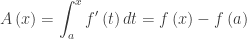
This equation is called the Fundamental Theorem of Calculus. In words, it says that the integral of a function can be found by evaluating the function of which the integrand is the derivative at the endpoints of the interval and subtracting the values. This is a number that may be positive, negative, or zero depending on the function and the interval. The function of which the integrand is the derivative, is called the antiderivative of the integrand.

The real meaning and use of the FTC is twofold:

It says that the integral of a rate of change (i.e. a derivative) is the net amount of change. Thus, when you want to find the amount of change – and you will want to do this with every application of the derivative – integrate the rate of change.
It also gives us an easy way to evaluate a Riemann sum without going to all the trouble that is necessary with a Riemann sum; simply evaluate the antiderivative at the endpoints and subtract.

At this point I suggest two quick questions to emphasize the second point:

Find $\int_{3}^{7}{{2xdx}}$ .

Ask if anyone knows a function whose derivative is 2x? Your students will know this one. The answer is x², so

$\displaystyle \int_{3}^{7}{{2xdx}}={{7}^{2}}-{{3}^{2}}=40$ .

Much easier than setting up and evaluating a Riemann sum!

2. Then ask your students to find the area enclosed by the coordinate axes and the graph of cos(x) from zero to $\frac{\pi }{2}$ . With a little help they should arrive at

$\displaystyle \int_{0}^{{\pi /2}}{{\cos \left( x \right)dx}}$ .

Then ask if anyone knows a function whose derivative is cos(x). it’s sin(x), so

$\displaystyle \int_{0}^{{\pi /2}}{{\cos \left( x \right)dx}}=\sin \left( {\frac{\pi }{2}} \right)-\sin \left( 0 \right)=1-0=1$ .

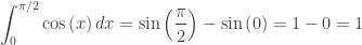
At this point they should be convinced that the FTC is a good thing to know.

There is another form of the FTC that is discussed in More About the FTC.

Good Question 11 – Riemann Reversed

Posted on November 29, 2016 by Lin McMullin

Good Question 11 – or not.

The question below appears in the 2016 Course and Exam Description (CED) for AP Calculus (CED, p. 54), and has caused some questions since it is not something included in most textbooks and has not appeared on recent exams. The question gives a Riemann sum and asks for the definite integral that is its limit. Another example appears in the 2016 “Practice Exam” available at your audit website; see question AB 30. This type of question asks the student to relate a definite integral to the limit of its Riemann sum. These are called reversal questions since you must work in reverse of the usual order. Since this type of question appears in both the CED examples and the practice exam, the chances of it appearing on future exams look good.

To the best of my recollection the last time a question of this type appeared on the AP Calculus exams was in 1997, when only about 7% of the students taking the exam got it correct. Considering that by random guessing about 20% should have gotten it correct, this was a difficult question. This question, the “radical 50” question, is at the end of this post.

Example 1

Which of the following integral expressions is equal to $\displaystyle \underset{n\to \infty }{\mathop{\lim }}\,\sum\limits_{k=1}^{n}{\left( \sqrt{1+\frac{3k}{n}}\cdot \frac{1}{n} \right)}$ ?

There were 4 answer choices that we will consider in a minute.

The first key to answering the question is to recognize the limit as a Riemann sum. In general, a right-side Riemann sum for the function f on the interval [a, b] with n equal subdivisions, has the form:

$\displaystyle \underset{n\to \infty }{\mathop{\lim }}\,\sum\limits_{k=1}^{n}{\left( f\left( a+\frac{b-a}{n}\cdot k \right)\cdot \frac{b-a}{n} \right)}=\int_{a}^{b}{f\left( x \right)dx}$

To evaluate the limit and express it as an integral, we must identify, a, b, and f. I usually begin by looking for $\displaystyle \frac{b-a}{n}$ . Here $\displaystyle \frac{b-a}{n}=\frac{1}{n}$ and from this conclude that b – a = 1, so b = a + 1.

Usually, you can start by considering a = 0 , which means that the $\displaystyle \frac{b-a}{n}\cdot k$ becomes the “x.”. Then rewriting the radicand as $\displaystyle 1+3\frac{1}{n}k=1+3\left( a+\frac{1}{n}\cdot k \right)$ , it appears the function is $\sqrt{1+3x}$ and the limit is $\displaystyle \int_{0}^{1}{\sqrt{1+3x}}dx=\frac{14}{9}$ .

The answer choices are

(A) $\displaystyle \int_{0}^{1}{\sqrt{1+3x}}dx$ (B) $\displaystyle \int_{0}^{3}{\sqrt{1+x}}dx$ (C) $\displaystyle \int_{1}^{4}{\sqrt{x}}dx$ (D) $\displaystyle \tfrac{1}{3}\int_{0}^{3}{\sqrt{x}}dx$

The correct choice is (A), but notice that choices B, C, and D can be eliminated as soon as we determine that b = a + 1. That is not always the case.

Let’s consider another example:

Example 2: $\displaystyle \underset{n\to \infty }{\mathop{\lim }}\,\sum\limits_{k=1}^{n}{\left( {{\left( 2+\frac{3}{n}k \right)}^{2}}\left( \frac{3}{n} \right) \right)}=$

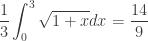
As before consider $\displaystyle \frac{b-a}{n}=\frac{3}{n}$ , which implies that b = a + 3. With a = 0, the function appears to be ${{\left( 2+x \right)}^{2}}$ on the interval [0, 3], so the limit is $\displaystyle \int_{0}^{3}{{{\left( 2+x \right)}^{2}}}dx=39$

BUT

What if we take a = 2? If so, the limit is $\displaystyle \int_{2}^{5}{{{x}^{2}}dx}=39$ .

And now one of the “problems” with this kind of question appears: the answer written as a definite integral is not unique!

Not only are there two answers, but there are many more possible answers. These two answers are horizontal translations of each other, and many other translations are possible, such as $\displaystyle \int_{-25.65}^{-22.65}{{{\left( 27.65+x \right)}^{2}}dx}=39$ .

The same thing can occur in other ways. Returning to example 1,and using something like a u-substitution, we can rewrite the original limit as $\displaystyle \frac{1}{3}\cdot \underset{n\to \infty }{\mathop{\lim }}\,\sum\limits_{k=1}^{n}{\left( \sqrt{1+\frac{3k}{n}}\cdot \frac{3}{n} \right)}$ .

Now b = a + 3 and the limit could be either $\displaystyle \frac{1}{3}\int_{0}^{3}{\sqrt{1+x}}dx=\frac{14}{9}$ or $\displaystyle \frac{1}{3}\int_{1}^{4}{\sqrt{x}}dx=\frac{14}{9}$ , among others.

My opinions about this kind of question.

The real problem with the answer choices to Example 1 is that they force the student to do the question in a way that gets one of the answers. It is perfectly reasonable for the student to approach the problem a different way, and get a different correct answer that is not among the choices. This is not good.

The problem could be fixed by giving the answer choices as numbers. These are the numerical values of the 4 choices:(A) 14/9 (B) 14/3 (C) 14/3 (D) $2\sqrt{3}/3$ . As you can see that presents another problem. Distractors (wrong answers) are made by making predictable calculus mistakes. Apparently, two predictable mistakes give the same numerical answer; therefore, one of them must go.

A related problem is this: The limit of a Riemann sum is a number; a definite integral is a number. Therefore, any definite integral, even one totally unrelated to the Riemann sum, which has the correct numerical value, is a correct answer.

I’m not sure if this type of question has any practical or real-world use. Certainly, setting up a Riemann sum is important and necessary to solve a variety of problems. After all, behind every definite integral there is a Riemann sum. But starting with a Riemann sum and finding the function and interval does not seem to me to be of practical use.

The CED references this question to MPAC 1: Reasoning with definitions and theorems, and to MPAC 5: Building notational fluency. They are appropriate,and the questions do make students unpack the notation.

My opinions notwithstanding, it appears that future exams will include questions like these.

These questions are easy enough to make up. You will probably have your students write Riemann sums with a small value of n when you are teaching Riemann sums leading up to the Fundamental Theorem of Calculus. You can make up problems like these by stopping after you get to the limit, giving your students just the limit, and having them work backwards to identify the function(s) and interval(s). You could also give them an integral and ask for the associated Riemann sum. Question writers call questions like these reversal questions since the work is done in reverse of the usual way.

Here is the question from 1997, for you to try. The answer is below.

Answer B. Hint n = 50

Revised 5-5-2022

Graphing Integrals

Posted on November 15, 2016 by Lin McMullin

The sixth in the Graphing Calculator / Technology series

The topic of integration is coming up soon. Here are some notes and ideas about the integration operation on graphing calculators. The entries are the same or very similar for all calculator brands.

The basic problem of evaluating a definite integral on a graphing calculator is done without finding an antiderivative; that is, the calculator uses a numerical algorithm to produce the result. The calculator provides a template,and you fill in the 4 squares so that the expression looks exactly like what you write by hand. Then the calculator computes the result. (Older models require a one-line input requiring, in order, the integrand, the independent variable, the lower limit of integration and the upper limit in that order, separated by commas.) The first interesting thing is that the variable in the integrand does to have to be x. As the first figure illustrates using x or a or any other letter gives the same result.

This is because the variable of integration is just a place holder. Sometimes called a “dummy variable”, this letter can be anything at all, including x. On the home or calculation screen you might as well always use x, so the entry will look like what you have on your paper. As we will see, when graphing it may be less confusing to use a different letter.

The antiderivative, F, of any function, f, can be written as a function defined by an integral where there is a point on the antiderivative of f , which is with F ’ = f. The point (a, F(a)) is the initial condition. (In the following we will use F(a) = 0 as the initial condition – the graph will contain the origin. As a further investigation, try changing the lower limit to different numbers and see how that changes the graph.)

The integration operation can be used to graph the antiderivative of a function without finding the antiderivative. You may graph the antiderivative when teaching antiderivatives. Have students look at the graph of the antiderivative and guess what that function is.

When graphing use x as the upper limit of integration and a different letter for the variable in the rest of the template. The calculator will use different values of x to calculate the points to be graphed.

The set-up shown in the next figure shows how to enter a function defined by an integral (blue line) and the same function obtained by antidifferentiating (red squares). As you can see the results are the same.

In this way, you can explore the functions and their indefinite integrals by graphing.

The Fundamental Theorem of Calculus

Another use of using the graph of an integral is to investigate both parts of the Fundamental Theorem of Calculus (FTC). Roughly speaking, the FTC says that the integral of a derivative of a function is that function, and the derivative of an integral is the integrand.

In the figure below, the same function is entered both ways; the graphs are the same. (Note the x’s in the second line must be x in all four places.)

Foreshadowing the FTC

Posted on December 15, 2014 by Lin McMullin

This is an example to help prepare students to tackle the Fundamental Theorem of Calculus (FTC). Use it after the lesson on Riemann sums and the definition of the definite integral, but before the FTC derivation.

Consider the area, A, between the graph of $f\left( x \right)=\cos \left( x \right)$ and the x-axis on the interval $\left[ 0,\tfrac{\pi }{2} \right]$ . Set up a Riemann sum using the general partition:

$0={{x}_{0}}<{{x}_{1}}<{{x}_{2}}<{{x}_{3}}<\cdots <{{x}_{n-2}}<{{x}_{n-1}}<{{x}_{n}}=\tfrac{\pi }{2}$

$\displaystyle A=\int_{0}^{{\scriptstyle{}^{\pi }\!\!\diagup\!\!{}_{2}\;}}{\cos \left( x \right)dx}=\underset{\Delta x\to 0}{\mathop{\lim }}\,\sum\limits_{i=1}^{n}{\cos \left( {{c}_{i}} \right)\left( {{x}_{i}}-{{x}_{i-1}} \right)}$

Since we can choose the value of ${{c}_{i}}$ any way we want, let’s take the same intervals and use ${{c}_{i}}$ the number guaranteed by the Mean Value Theorem for the function $F\left( x \right)=\sin \left( x \right)$ on the each sub-interval interval. That is, on each sub-interval at $x={{c}_{i}}$

$\left. \frac{d}{dx}\sin \left( x \right) \right|_{x={{c}_{i}}}^{{}}=\cos \left( {{c}_{i}} \right)=\frac{\sin \left( {{x}_{i}} \right)-\sin \left( {{x}_{i-1}} \right)}{\left( {{x}_{i}}-{{x}_{i-1}} \right)}$

Then, substituting into the Riemann sum above

$\displaystyle A=\underset{\Delta x\to 0}{\mathop{\lim }}\,\sum\limits_{i=1}^{n}{\cos \left( {{c}_{i}} \right)\left( {{x}_{i}}-{{x}_{i-1}} \right)}=\underset{\Delta x\to 0}{\mathop{\lim }}\,\sum\limits_{i=1}^{n}{\frac{\sin \left( {{x}_{i}} \right)-\sin \left( {{x}_{i-1}} \right)}{\left( {{x}_{i}}-{{x}_{i-1}} \right)}\left( {{x}_{i}}-{{x}_{i-1}} \right)}$

$\displaystyle A=\underset{\Delta x\to 0}{\mathop{\lim }}\,\sum\limits_{i=1}^{n}{\left( \sin \left( {{x}_{i}} \right)-\sin \left( {{x}_{i-1}} \right) \right)}$

Now writing out the terms we have a telescoping series:

$\displaystyle A=\left( \sin \left( {{x}_{1}} \right)-\sin \left( {{x}_{0}} \right) \right)+\left( \sin \left( {{x}_{2}} \right)-\sin \left( {{x}_{1}} \right) \right)+\left( \sin \left( {{x}_{3}} \right)-\sin \left( {{x}_{2}} \right) \right)+$

$\displaystyle \cdots +\left( \sin \left( {{x}_{n-1}} \right)-\sin \left( {{x}_{n-2}} \right) \right)+\left( \sin \left( {{x}_{n}} \right)-\sin \left( {{x}_{n-1}} \right) \right)$

$\displaystyle A=\sin \left( {{x}_{n}} \right)-\sin \left( {{x}_{0}} \right)$

$\displaystyle A=\sin \left( \tfrac{\pi }{2} \right)-\sin \left( 0 \right)=1$

As you can see, this is really just the derivation of the FTC applied to a particular function. Now the students should have a better idea of what’s going on when you solve the problem in general, i.e. when you prove the FTC.

More About the FTC

Posted on December 19, 2012 by Lin McMullin

In keeping with my idea from the last post of sneaking up on ideas, here is a way to sneak up on the other part of the FTC.

Consider these three functions F1(t) = 3, F2(t) = 2t and F3(t) = 2t + 3

For each of these three functions do the following:

Graph each function on the interval [0, t] for $t\ge 0$ .
Let x be a value of t and let x move to the right along the t-axis starting at zero. Using area formulas, write functions, A1(x), A2(x), and A3(x), for the areas of the region between the graph and the t-axis. Make a table of values for x = 1, 2, 3, …, 10. Do not use any “calculus”; the area expressions are easy to find from geometry. (A1(t) = 3t; A2(t) = t²; A3(t) = t²+ 3t )
Consider what happens as the as x moves from zero to the right. The expressions are a function that gives the area for each x. Now write expressions for the three areas with an integral that gives the same area. The lower limit will be 0 and the upper limit will be x.
These are examples of functions defined by integrals. Each different value of x as the upper limit of integration, will give a unique value (area).
Differentiate the area functions and compare them to the functions from which they came. What do you notice?

Consider the FTC where the integral has an upper limit of x. That is, a function defined by an integral. (The lower limit does not have to be zero.)

$\displaystyle A\left( x \right)=\int_{a}^{x}{{f}'\left( t \right)dt}=f\left( x \right)-f\left( a \right)$

What is ${A}'\left( x \right)$ ?

$\displaystyle {A}'\left( x \right)=\frac{d}{dx}\int_{a}^{x}{{f}'\left( t \right)dt}=\frac{d}{dx}\left( f\left( x \right)-f\left( a \right) \right)={f}'\left( x \right)-0$

$\displaystyle \frac{d}{dx}\int_{a}^{x}{{f}'\left( t \right)dt}={f}'\left( x \right)$

The is the other part of the FTC which says that the derivative of a function defined by an integral is the integrand, f (x) evaluated at x.

A good way to demonstrate this to your students is to do a simple integral like

$\displaystyle \int_{\pi /4}^{x}{\cos \left( t \right)dt}=\sin \left( x \right)-\tfrac{\sqrt{2}}{2}$ ,

and then differentiate to show that

$\displaystyle \frac{d}{dx}\int_{\pi /4}^{x}{\cos \left( t \right)dt}=\frac{d}{dx}\left( \sin \left( x \right)-\tfrac{\sqrt{2}}{2} \right)=\cos \left( x \right)$

This part of the FTC says, roughly, very roughly, that the derivative of an integral is this integrand. The other part, discussed in the last post, just as roughly, says the integral of the derivative is the antiderivative.

Keep your notes on this activity. In my next post I will use these functions to demonstrate some of the important properties of integrals.

The Fundamental Theorem of Calculus

Posted on December 17, 2012 by Lin McMullin

The Fundamental Theorem of Calculus or FTC, as its name suggests, is a very important idea. It is not sufficient to present the formula and show students how to use it. Show them where it comes from.

Here is an approach to demonstrate the FTC. I try to sneak up on the result by proposing a problem and then solving it. Here is the outline.

Suppose we have a differentiable function f that goes from $\left( a,f\left( a \right) \right)$ to $\left( b,f\left( b \right) \right)$ . What is the net change in f over this interval? Easy it’s $f\left( b \right)-f\left( a \right)$ . No problem, but way too easy for a calculus class. So let’s try a harder way!

Partition the interval [a, b] as you would for a Riemann sum, and calculate the change in f on each subinterval. The subintervals may be the same width or not. The change in y on the general subinterval [x_i_-1, x_i] is $f\left( {{x}_{i}} \right)-f\left( {{x}_{i-1}} \right)$ .

Approximate the net change over the whole interval by adding these $\displaystyle \sum\limits_{i=1}^{n}{\left( f\left( {{x}_{i}} \right)-f\left( {{x}_{i-1}} \right) \right)}$ .
Is this a Riemann sum? No it is not! There is no $\Delta x$ part. What to do?

The expression $f\left( {{x}_{i}} \right)-f\left( {{x}_{i-1}} \right)$ looks familiar.
It is part of the equation for the Mean Value Theorem: $\displaystyle {f}'\left( c \right)=\frac{f\left( b \right)-f\left( a \right)}{b-a}$ or ${f}'\left( c \right)\left( b-a \right)=f\left( b \right)-f\left( a \right)$ .
If we adapt this to the subinterval letting c_i be the number guaranteed by the MVT on each subinterval [x_i_-1, x_i], then $f\left( {{x}_{i}} \right)-f\left( {{x}_{i-1}} \right)={f}'\left( {{c}_{i}} \right)\left( {{x}_{i}}-{{x}_{i-1}} \right)$

We can rewrite the sum in step 3 as $\displaystyle \sum\limits_{i=1}^{n}{\left( f\left( {{x}_{i}} \right)-f\left( {{x}_{i-1}} \right) \right)}=\sum\limits_{n=1}^{n}{\left( {f}'\left( {{c}_{i}} \right)\left( {{x}_{i}}-{{x}_{i-1}} \right) \right)}$ .

This is a Riemann sum and therefore, $\displaystyle \underset{n\to \infty }{\mathop{\lim }}\,\sum\limits_{n=1}^{n}{\left( {f}'\left( {{c}_{i}} \right)\left( {{x}_{i}}-{{x}_{i-1}} \right) \right)}=\int_{a}^{b}{{f}'\left( c \right)dx}$ .
So what is this equal to? We have already found what this limit is in step 1, so we now have:

$\displaystyle \int_{a}^{b}{{f}'\left( x \right)dx}=f\left( b \right)-f\left( a \right)$ .

This is called the FTC. And it is important.

The first thing it tells us is that the integral of a rate of change is the (net) amount of change. This will help us do a variety of problems.

The second thing it tells us is that, if we can find a function of which the integrand is the derivative (i.e. its antiderivative), then we can find the value of a definite integral by evaluating an antiderivative at the endpoints and subtracting. No more struggling with trying to find the limit of Riemann sums or graphing the function and hoping you can break it into regions with easy to find areas. All we need is an antiderivative and then one quick computation will do the trick from now on.

There is more to the FTC. This will be the subject of the next post.

The Definition of the Definite Integral

Posted on December 14, 2012 by Lin McMullin

From the last post, it seems pretty obvious that as the number of rectangles in a Riemann sum increases or, what amounts to the same thing, the width of the sub-intervals decreases, the Riemann sum approaches the area of the region between a graph and the x-axis. The figures below show left-Riemann sums for the function $f\left( x \right)=1+{{x}^{2}}$ on the interval [1, 4]. Hover and click on the figure below.

This slideshow requires JavaScript.

As the number of rectangles increases, they fill up more and more of the region. The sums increase, yet, their sum is always less than the area. They form an increasing sequence which is bounded above and therefore approaches its least upper bound (the area) as a limit.

Right-side rectangles work almost the same way. The sums form a decreasing sequence that is bounded below by the area and thus they approach the same limit.

All of the other Riemann sums must be between these two (at least for this example) and thus all approach the same limit.

This limit is called the definite integral for f on the interval [a, b], denoted by the new symbol below.

$\displaystyle \underset{n\to \infty }{\mathop{\lim }}\,\sum\limits_{i=1}^{n}{f\left( x_{i}^{*} \right)\left( {{x}_{i}}-{{x}_{i-1}} \right)}=\underset{\Delta x\to 0}{\mathop{\lim }}\,\sum\limits_{i=1}^{n}{f\left( x_{i}^{*} \right)\Delta x=\int_{a}^{b}{f\left( x \right)dx}}$

The notation has the advantage of being simpler to write than all the limit stuff and it shows us the interval which the limits do not. (For now consider the dx as a stand-in for $\Delta x$ .)

The disadvantage of the notation is that, as we use it for real applications, the concept of Riemann sums often gets lost. The integrals become formulas and they get memorized but not understood.

Remember: behind every (any, all) definite integral is a Riemann sum. As we look at applications, we should always look for the Riemann sum and how it is set up. This will tell us what the definite integral should be. We will not need to be too fussy about the subscripts and such; in fact, we will almost ignore them, but we will look carefully at the Riemann sum rectangles.

Teaching Calculus

The pleasure lies not in discovering the truth, but in searching for it.

Tag Archives: FTC

The Definite Integral and the FTC

Good Question 11 – Riemann Reversed

Graphing Integrals

Foreshadowing the FTC

More About the FTC

The Fundamental Theorem of Calculus

The Definition of the Definite Integral

Share this:

Share this:

Share this:

Share this:

Share this:

Share this:

Share this: