This blog post describes a lesson that investigates some ideas about sequences that are not stressed in the AP Calculus curriculum. The lesson could be an introduction to sequences. I think the lesson would work in an Algebra I course and is certainly suitable for a pre-calculus course. The investigation is of irrational numbers and their decimal representation. The successive decimal approximations to the square root of 2 is an example of a non-decreasing sequence that is bounded above and therefore converges.
Students do not need to know any of that as it will be developed in the lesson. Specifically, don’t even mention square roots, the square root of 2, or even irrational numbers until a student mention something of the sort.
This is not an efficient algorithm for finding square roots. There are far more efficient ways.
We begin with some preliminaries.
Preliminaries
- There is a blank table that you can copy for students to use here.
- There is a summary of the new terms used and completed table Sequence Notes. Do not give this out until after the lesson is completed.
- We will be working with some rather long decimal numbers that will need to be squared. Scientific and graphing calculators usually compute with 14 digits and give their results rounded to 12 digits. Since ours will quickly get longer than that, I suggest you use WolframAlpha. This can be used with a computer online (at wolframalpha.com) or with an app available for smart phones and tablets. It is best if students have this website or app for their individual use.
Students will enter their numbers as shown below. Specifying “30 digits” will produces answers long enough for our purpose. To speed things up, students can edit the current number by changing the last digit in the entry line. When you get started you may have to show students how to do this. Students will need internet access.
Computer Smart phone
The Lesson
The style of the lesson is Socratic. You, the teacher, will present the problem, explain how they are to go about it, and ask leading questions as appropriate. Some questions are suggested; be ready to ask others. Later, you will have to explain (define) some new words, but as much as possible let the class suggest what to do. Drag things out of them, rather than telling them.
To begin – Produce some data
Explain to the class that they are going to generate and investigate two lists of numbers (technically called sequences). Each new member of the lists will be a number with one more decimal place than the preceding number.
The first list, whose members are called Ln, will be the largest number with the given number of decimal places, n, whose square is less than two. The subscript, n, stands for the number of decimal places in the number.
Ask: “What is the largest integer whose square is less than 2?” Answer 1, so, L0 = 1. Ask: What is the largest one place decimal whose square is less than 2?” Answer L1 =1.4.
The second list, Gn, will be the smallest number whose square is greater than 2. So, G0 = 2 and G1 = 1.5. Notice that 1.42 = 1.96 < 2 and 1.52 = 2.25 > 2
Divide the class into 10 groups named Group 0, Group 1, Group 2, …, Group 9. In each round the groups will append their “name” to the preceding decimal and square the resulting number. Group 0 squares 1.40, group 1, squares 1.41, group 2 squares 1.42, etc. using WolframAlpha.
Ask which groups have squares less than two and enter the largest in Ln, the next number will be the smallest number whose square is greater than 2; enter it in Gn.
Complete the table by entering the largest number whose square is less than 2 in the Ln column and the smallest number whose square is greater than 2 in the Gn column. At each stage, each group appends their digit to the most recent Ln . Project or write the table on the board. Students may fill in their own copy. A completed table is here: Sequence Notes and definitions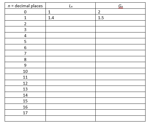
Next – Lead a discussion
When the table is complete, prompt the students to examine the lists and come up with anything and everything they observe whether it seems important or not. Accept and discuss each observation and let the others say what they think about each observation. (Obviously, don’t deprecate or laugh at any answer – after all at this point, we don’t know what is and is not significant.)
There are (at least) three observations that are significant to what we will consider next. Hopefully, someone will mention them; keep questioning them until they do. They are these, although students may use other terms:
- Ln is non-decreasing. Students may first say Ln is increasing. Pause if they do and look at L12 and L13, and L15 and L16. Ask how they know Ln is non-decreasing (because each time we add a digit on the end, you get a bigger number).
- Likewise, Gn is non-increasing.
- For all n, Ln < Gn, and the numbers differ only in the last digit, and with the last digits differing by 1.
Direct instruction: Explain these ideas and terms (definition)
- A sequence is a list or set of numbers in a given order.
- A sequence is bounded above if there exists a number greater than or equal to all the terms of the sequence. The smallest upper bound of a sequence is called its least upper bound (l.u.b.)
- A sequence is bounded below if there exists a number less than or equal to all the terms of the sequence. The largest lower bound is called the greatest lower bound (g.l.b.)
More questions: Apply these terms to the sequence Ln with questions like these:
- Is Ln bounded above, below, or not bounded? (Bounded above)
- Give an example of a number greater than all the terms of Ln. (Many answers: 1,000,000, 4, 2, 1.415, etc. and, in fact, any and every number in Gn)
- What is the l.u.b. of Ln? Can you think of the smallest number that is an upper bound of this sequence? (Yes,
 . Don’t tell them this – drag it out of them if necessary.) Why? How do you know this?
- Make the class convince you that for all n,

Ask similar questions about Gn.
- Is Gn bounded above, below, or not bounded? (Bounded below)
- Give an example of a number less than all the terms of Ln. (Many answers: any negative number, zero, 1, 1.414, etc. Any and every number in Ln)
- What is the g.l.b. of Gn? Can you think of the greatest number that is a lower bound of this sequence? (Yes, ) Why? How do you know this?
- Make the class convince you that for all n,

Summing Up
Ask, “What’s happening with the numbers in the Ln sequence?” and “What’s happening to the numbers in the Gn sequence?”
The answer you want is that they are getting closer to , one from below, the other from above. (As always, wait for a student to suggest this and then let the others discuss it.)
Once everyone is convinced, explain how mathematicians say and write, “gets closer to”:
Mathematicians say that is the limiting value (or limit) of both sequences. They write and .
Explain very carefully that while  is read, “n approaches infinity,” that infinity,
  , is not a number. The symbol means that n gets larger without bound or that n gets larger than all (any, every) positive numbers.
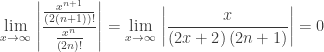
In a more technical sense there is an infinite series  where
where  is one of the digits 0, 1, 2, 3, …, 9, but there is no formula for listing the values of . However, the sequence of partial sum of this series is the sequence
  which converges to
  . Therefore,
is an Irrational number, but this same procedure may be used to find decimal approximation of roots of rational numbers as well. However, for Rational numbers, there are easier ways.
Finally, Irrational numbers are exactly those that cannot be written as repeating (or terminating) decimals. They “go on forever” with no pattern. The decimals you can calculate eventually stop and are rounded to the last digit. Even WolframAlpha and similar computers must eventually do this. Irrational numbers are the limits of sequences like the one we looked at today.
Exercises
- Follow the procedure above to find the sequence whose limit is
 . Find this number the usual way (simplify and use long division) and compare the results.
- Follow the procedure above to find the sequence whose limit is
 . Find this number the usual way and compare the results.
- Using WolframAlpha determine if the computer is using Ln, Gn. both, or neither when it gives a value for . (Hint: enter “square root 2 to 5 digits” and change to 6, 7, and 8 digits; compare the answer with the sequences, you found.)
Answers:
- 0.363636…
- 0.625
- For n = 5 and 6 the numbers are from Ln, for n = 7 and 8 they are from Gn. WolframAlpha is using a different algorithm to compute the square root of 2; the numbers appear from both sequences due to the rounding of the answers. To see WolframAlpha’s algorithm type “square root algorithm” on the entry line. This method also produces a sequence of approximations a/b.
Revised July 28, 2021


 , sin(x), cos(x), and ex
 ; if a = 0, the series is called a Maclaurin series.
 and be able to find other series by substituting into one of these.
 . Re-writing a rational expression as the sum of a geometric series and then writing the series has appeared on the exam.
 )
) , which I found curious.
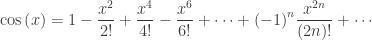
 for x gives

 is a Real number. In addition, since the function ends at x = 0, how can the Maclaurin series be centered there? Since it is not defined to the left of zero, how can it have derivatives at zero?
 in red largely covered by its Maclaurin series (with n = 14) in blue.
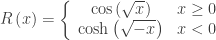
 )
) and 5/17 may look “exact,” but if you ever had to measure something to those values, you’re back to using decimal approximations.


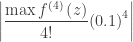 for some number z between 0 and 0.1.

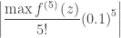 to calculate the error bound. The 5th derivative of the sin(x) is cos(x) and its maximum value in the range is cos(0) =1.

