The Fundamental Theorem of Calculus is, well, fundamental. It relates the derivative and the integral.
Writing a Riemann sum with all that fancy notation is tedious. To speed things up a special notation is used to replace it. The limit of the Riemann sum for a function on an interval [a, b] is written as its definite integral:
The (called the integrand) is the function with no fancy notation and the dx, called differential x replaces the . The a and b, called the lower and upper limit of integration respectively, show you the interval the Riemann sum was formed on (which the Riemann sum does not).
Keep in mind that behind every definite integral is a Riemann sum. Therefore, all the properties of limits apply to definite integrals. They can be added and subtracted, a constant may be factored out, and so on.
The Fundamental Theorem of Calculus, the FTC, tells you how to evaluate a definite integral (and therefore its Riemann sum): Simply evaluate the function of which is the derivative at the endpoints of the interval and subtract.
To keep this in mind you can write the FTC like this considering the integrand as the derivative (of something):
.
For example, since ,
That’s all there is to it!
But wait! There’s more! This reveals another important idea: Since derivatives are rates of change, the FTC says that the integral of a rate of change is the net amount of change over the interval. Also called the accumulated change.
Well, okay, there is the problem of finding the function whose derivative is the integrand which is not always easy. This function is called theantiderivative of the integrand; another name is the indefinite integral. (The notation for an antiderivative or indefinite integral is the same as for a definite integral without the limits of integration). The truth is that finding the antiderivative is not as straightforward as finding the derivative. We will tackle that soon.
We are now at the point where we can look at a special technique for finding some limits. Graph on your calculator y = sin(x) and y = x near the origin. Zoom in a little bit. The line is tangent to sin(x) at the origin and their values are almost the same. Look at the two graphs near the origin and see if you can guess the limit of their ratio at the origin: ?.
In this example, if you substitute zero into the expression you get zero divided by zero and there is no way to divide out the zero in the dominator as you could with rational expressions.
This kind of thing is called an indeterminate form. The limit of an indeterminate form may have a value, but in its current form you cannot determine what it is. When you studied limits, you were often able to factor and divide out the denominator and find the limit for what was left. With you can’t do that.
But by replacing the expressions with their local linear approximations, the offending factor will divide out leaving you with the ratio of the derivatives (slopes). This limit may be easier to find.
The technique is called L’Hospital’s Rule, after Guillaume de l’Hospital (1661 – 1704) whose idea it wasn’t! He sort of “borrowed’ it from Johann Bernoulli (1667 – 1784).
L’Hospital’s Rule gives you a way of finding limits of indeterminate forms. You will look at indeterminate forms of the types and . The technique may be expanded to other indeterminate forms like which are not tested on the AP Calculus exams.
Like other “rules” in math, L’Hospital’s Rule is really a theorem. Before you use it, you must check that the hypotheses are true. And on the AP Calculus exams you must show in writing that you have checked.
We would like to study nice well-behaved functions; functions that are smooth and that don’t do strange things. Yeah, well good luck with that.
One of the things that might be nice is that you could draw the graph of a function from one end of its domain to the other without taking your pen off the paper. And a lot of functions are like that, but not all.
Some functions have holes in them, others jump from one y-value to another without hitting points in between. Some “go off to infinity” and come right back; others go off the top of the graph and come back from the bottom. Some go really crazy around a point.
Functions that you can draw from one end of their domain to the other without lifting your pen are said to be continuous.
More mathematically: A function is continuous at a point (that is, at a single value of x) if, and only if, as you travel along the graph towards the value (from either side of the x-value), the y-values on the graph are approaching the y-value at the point. In symbols: .
A function is continuous on an interval if, and only if, it is continuous at every value in the interval.
Wait! What?? I have to check all the points??
Technically, yes; practically, no. Most of the time you can easily show that a function is continuous everywhere by looking at its limit in general.
Moreover, you will learn to see where a function is not continuous. This is an important skill: looking at a function and suspecting there is a problem with continuity.
Take a quick look at some of the problems that functions may have at a point. Graph these on your calculator. They all have a “problem” at x = 3. Graph each example and you will see what they look like. Try to figure out why they have a “problem” and what causes it.
.
. This function has a single hole in the graph at (3, 3); It one may be difficult to see. Try using ZDecimal. A single point is missing because there is no value at x= 3 because the denominator is zero.
.
Zoom in several times at (3, 0) where the function has no value.
Learn to suspect that a function may have a discontinuity. (It’s not always at x = 3) The problem is often a zero denominator.
This is not just a game or some curious functions. One of the main tools of calculus called the derivative, which you will study next, is defined as the limit of a special function which is never continuous at the point you are interested in.
First, right from the start: Infinity is NOT a number.
Lots of folks think of infinity as the largest number possible, greater than anything else. That’s understandable because infinity, denoted by the symbol , is often used that way by those unlucky folks who don’t understand mathematics.
We’ll start with an example: Consider the fraction . This fraction has no value when x = 3 because there the denominator is zero. And you cannot divide by zero. Nothing personal, no one, no matter how smart, can divide by zero. Ever. Permanently and forever not allowed. Don’t even think about it! (Actually, think about it; just don’t do it.)
What you should say in such cases is that the expression has no value, or is “undefined,” or “the limit does not exist,” abbreviated DNE.
In situations like the example we say, “the limit of the fraction as x approaches 3 equals infinity,” abbreviated . This means that the expression gets larger as x gets closer to three. The expression will be greater than any (large) number you want, if you are close enough to three.
You don’t believe me? Okay pick a large number, maybe . I say pick any value for x between 2.9999 and 3.0001 () and the expression will be larger than . Try it on your calculator.
How about ? Try a number between 2.9999999999 and 3.0000000001. I can play this game all day.
Try graphing the on your calculator. (Hint: Whenever you come across something like this, it is a great idea to graph the expression on your graphing calculator. Graphs can help you see what’s going on. Keep that in mind for the future.)
That’s the way to think about infinity: Infinity is what you say when you’re working with an expression that grows greater than any number you choose.
You may also use infinity to say what happens all the way to the left or right of the graph, its end behavior. The variable, x, may “approach infinity,” that is x moves further to the right (or is greater than any number you choose) the fraction above gets closer to zero: .
You may not do arithmetic with infinity.
Arithmetic is for numbers.
You will see a number of expressions whose limit is equal to infinity, like . Which really means, just what we saw above: that as you (not “you” but x) get closer to 3, the value of the expression will be greater than any number you pick. The symbol is a shorthand way of saying this.
The opposite of infinity, , sometimes called “negative infinity,” means that the expression gets less than (i.e. more negative), than any negative number you choose.
Even though the expression has no limit, you are allowed to say the limit equals infinity. That’s funny when you think about it. It might be better if everyone said “undefined” or DNE, but they don’t. What can I say?
A word of warning: You may only say “equals infinity” is situations like the example above.
There are other similar expressions that have no limit where it is incorrect to say the limit equals infinity. For example,
has no value, is “undefined,” when x = 0, but . (Hint: this is where you should look at a graph on your graphing calculator to see why.)
does not exist. This is very similar to the first example but look at the graph and you’ll see a big difference.
So, good luck and enjoy your limitless journey through the infinite reaches of calculus. (Oh, wait! Can I say that?)
Your journey into calculus starts with the topic of limits. Why? Because limits make calculus work. The two big things in calculus are called the derivative and the definite integral; both are limits.
The first use of limits will be when you study continuity. A continuous function is one, roughly speaking, whose graph can be drawn without taking your pen off the paper. Limits will make this concept firm mathematically.
After that, if you flip through your book, you won’t see that many limits after the limit chapter. You will see derivatives and definite integrals – they are limits under a different name.
Notation: There is a new notation to learn for limits. It looks like this . This is read, “The limit as x approaches 6 of the sine of π divided by 6 equals ½.”
You will start by finding the limits of various functions. Sometimes the limit is easy to find – just substitute the number x is approaching into the (that’s what happened above); what you get is the limit. If a limit exists, it is a number. If you get a number by substituting, usually that’s the limit – end of problem.
But other times you get expressions that are not numbers when you substitute (like maybe you end up trying to divide by zero). In that case, you will need to do some sort of algebraic or trigonometric simplification. Your teacher will help you learn the “tricks” involved. Derivatives and the definite integral are both limits involving dividing by zero.
Some limits may not exist at all; in this case, you say, “Does not exist” or “DNE.” Others do not exist, but we say they are “equal to infinity.” Infinity will be the subject of the next post in this series.
As you learn to find limits, look for patterns. The limits of similar looking expressions are often found in similar ways.
One good way to see what a limit is, or is not, is to graph the expression. Use your graphing calculator.
Your calculator may “misinform” you sometimes! But even that is a help. (Hint: when your calculator does misinform you, about limits or anything else, that’s a time to look deeper into the situation: something interesting is going on.)
Producing a table of values (on your calculator) can often help you see what’s happening, as well. (Hint: while tables are useful, what happens between the values in the table is not always clear; that’s where the trouble may be.)
The first thing you will use limits for is to investigate continuity. When limits do not exist, continuity is usually the problem. Continuity will be the subject of a later post.
So, get ready for your trip through calculus: it’s an unlimited journey.
The next post in this series, “Why Infinity?”, will appear on Friday August 25, 2023.
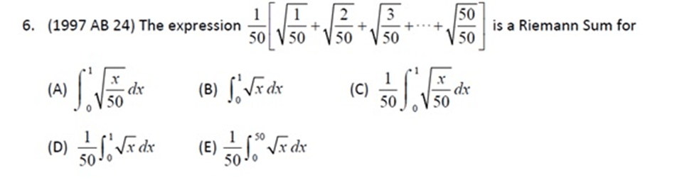
The question below appears in the new Course and Exam Description (CED) for AP Calculus, and has caused some questions since it is not something included in most textbooks and has not appeared on recent exams.
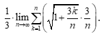
Example 1
Which of the following integral expressions is equal to
There were 4 answer choices that we will consider in a minute.
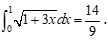
To the best of my recollection the last time a question of this type appeared on the AP Calculus exams was in 1997, when only about 7% of the students taking the exam got it correct. Considering that by random guessing about 20% should have gotten it correct, this was a difficult question. This question, the “radical 50” question is at the end of this post.
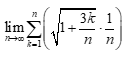
The first key to answering the question is to recognize the limit as a Riemann sum. In general, a right-side Riemann sum for the function f on the interval [a, b] with n equal subdivisions has the form:
To evaluate the limit and express it as an integral, we must identify, a, b, and f. I usually begin by looking for (b – a)/n. In this problem (b – a)/n = 1/n and from this conclude that b – a = 1, so b = a + 1.
Then rewriting the radicand as
It appears that the function is
and the limit is
.This is the first answer choice. The choices are:
In this example, choices B, C, and D can be eliminated as soon as we determine that b = a + 1, but that is not always the case.
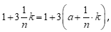
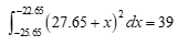
Let’s consider another example:
Example 2:
As before consider (b – a)/n = 3/n implies that b = a + 3. And the function appears to be
on the interval [0, 3], so the limit is
BUT
What is we take a = 2. If so, the limit is
And now one of the “problems” with this kind of question appears: the answer written as a definite integral is not unique!
Not only are there two answers, but there are many more possible answers. These two answers are horizontal translations of each other, and many other translations are possible, such as
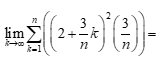
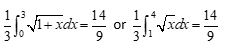
Returning to example 1, using something like a u-substitution, we can rewrite the original limit as .
Now b = a + 3 and the limit could be either
You will probably have your students write Riemann sums with a small value of n when you are teaching Riemann sums leading up to the Fundamental Theorem of Calculus. You can make up problems like this these by stopping after you get to the limit, giving your students just the limit, and have them work backwards to identify the function(s) and interval(s). You could also give them an integral and ask for the associated Riemann sum. Question writes call a question like this a reversal question, since the work is done in reverse of the usual way.
Another example appears in the 2016 “Practice Exam” available at your audit website. It is question AB 30. That question gives the definite integral and asks for the associate Riemann sum; a slightly different kind of reversal. Since this type of question appears in both the CED examples and the practice exam, chances of it appearing on future exams look good.
Critique of the problem
I’m not sure if this type of problem has any practical or real-world use. Certainly, setting up a Riemann sum is important and necessary to solve a variety of problems. After all, behind every definite integral there is a Riemann sum. But starting with a Riemann sum and finding the function and interval does not seem to me to be of practical use.
The CED references this question to MPAC 1: Reasoning with definitions and theorems, and to MPAC 5: Building notational fluency. They are appropriate, but still is the question ever done outside a test or classroom setting?
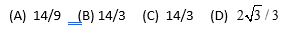
Another, bigger, problem is that the answer choices to Example 1 force the student to do the problem in a way that gets one of the answers. It is perfectly reasonable for the student to approach the problem a different way, and get another correct answer that is not among the choices. This is not good. The question could be fixed by giving the answer choices as numbers. These are the numerical values of the 4 choices:
As you can see that presents another problem.
Finally, here is the question from 1997, for you to try:
Answer B. Hint n = 50
_______________________________
Note: The original of this post was lost somehow. I’ve recreated it here. Sorry if anyone was inconvenienced. LMc May 5, 2024
Given equations that define a region in the plane students are asked to find its area, the volume of the solid formed when the region is revolved around a line, and/or the region is used as a base of a solid with regular cross-sections. This standard application of the integral has appeared every year since year one (1969) on the AB exam and almost every year on the BC exam. You can be fairly sure that if a free-response question on areas and volumes does not appear, the topic will be tested on the multiple-choice section.
What students should be able to do:
Find the intersection(s) of the graphs and use them as limits of integration (calculator equation solving). Write the equation followed by the solution; showing work is not required. Usually, no credit is earned until the solution is used in context (e.g., as a limit of integration). Students should know how to store and recall these values to save time and avoid copy errors.
Find the area of the region between the graph and the x-axis or between two graphs.
Find the volume when the region is revolved around a line, not necessarily an axis or an edge of the region, by the disk/washer method. See “Subtract the Hole from the Whole”
The cylindrical shell method will never be necessary for a question on the AP exams but is eligible for full credit if properly used.
Find the volume of a solid with regular cross-sections whose base is the region between the curves. For an interesting variation on this idea see 2009 AB 4(b)
Find the equation of a vertical line that divides the region in half (area or volume). This involves setting up an integral equation where the limit is the variable for which the equation is solved.
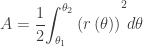
For BC only – find the area of a region bounded by polar curves:
For BC only – Find perimeter using arc length integral
If this question appears on the calculator active section, it is expected that the definite integrals will be evaluated on a calculator. Students should write the definite integral with limits on their paper and put its value after it. It is not required to give the antiderivative and if a student gives an incorrect antiderivative, they will lose credit even if the final answer is (somehow) correct.
There is a calculator program available that will give the set-up and not just the answer so recently this question has been on the no calculator allowed section. (The good news is that in this case the integrals will be easy, or they will be set-up-but-do-not-integrate questions.)
Occasionally, other type questions have been included as a part of this question. See 2016 AB5/BC5 which included an average value question and a related rate question along with finding the volume.
Shorter questions on this concept appear in the multiple-choice sections. As always, look over as many questions of this kind from past exams as you can find.


 ?.
?. you can’t do that.
  and
and  . The technique may be expanded to other indeterminate forms like
  which are not tested on the AP Calculus exams.
 .
. .
.
 . This function has a single hole in the graph at (3, 3); It one may be difficult to see. Try using ZDecimal. A single point is missing because there is no value at x= 3 because the denominator is zero.
 .
. Zoom in several times at (3, 0) where the function has no value.
 , is often used that way by those unlucky folks who don’t understand mathematics.
 . This fraction has no value when x = 3 because there the denominator is zero. And you cannot divide by zero. Nothing personal, no one, no matter how smart, can divide by zero. Ever. Permanently and forever not allowed. Don’t even think about it! (Actually, think about it; just don’t do it.)
 . This means that the expression gets larger as x gets closer to three. The expression will be greater than any (large) number you want, if you are close enough to three.
 . I say pick any value for x between 2.9999 and 3.0001 (
 ) and the expression will be larger than
  ? Try a number between 2.9999999999 and 3.0000000001. I can play this game all day.
 on your calculator. (Hint: Whenever you come across something like this, it is a great idea to graph the expression on your graphing calculator. Graphs can help you see what’s going on. Keep that in mind for the future.)
 .
.

 , sometimes called “negative infinity,” means that the expression gets less than (i.e. more negative), than any negative number you choose.
  has no value, is “undefined,” when x = 0, but
  . (Hint: this is where you should look at a graph on your graphing calculator to see why.)
 does not exist. This is very similar to the first example but look at the graph and you’ll see a big difference.
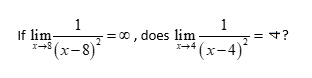
 . This is read, “The limit as x approaches 6 of the sine of π divided by 6 equals ½.”