This is the second in an occasional series on adapting and expanding AP calculus exam questions. Variations on multiple-choice questions may make other multiple-choice questions, or, if you do not like making up all the “wrong” choices they can be changed to short answer questions for use in your class homework or test. Other variations make for good discussion questions.
Today we will take a look at 2008 AB 10. This question gave the graph below and asked which of  , a left, right, or midpoint Riemann sum approximation, or a trapezoidal sum approximation of the integral all with four subintervals of equal length has the least value.
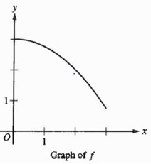
I’ll refer to these as I, L, R, M and T. The answer is R as a quick sketch will show.
In the discussion we will assume the curve does not change direction or concavity over the interval of integration. The answers to the questions in the variations are at the end of this post.
Variation 1: The question seems pretty easy so let’s beef it up a bit. How about asking the student to put I, L, R, M and T in order from smallest to largest? For a multiple-choice question answer choices are inequalities with all 5 sums in them.
The midpoint Riemann sum may be the most difficult to see. Here is the way to explain it. See the figure below.
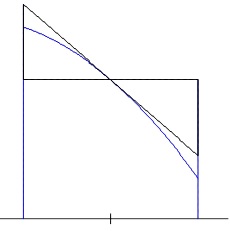
On each subinterval draw the horizontal segment at the function value at the midpoint of the interval. At this same point draw a tangent segment from one side of the interval to the other. This forms two congruent triangles with the horizontal segment and the edges of the interval.
Therefore, this midpoint trapezoid and the midpoint rectangle have the same area. Then because of the concavity, we see that in this case the midpoint Riemann sum, M, will be larger than the integral, I. With the same concavity the trapezoidal approximation will lie below the curve and therefore T < I < M. This will be true for any curve that is concave down. The opposite is true for a curve that is concave up: M < I < T. M and T are always on opposite sides of I.
Variation 2: Change the number of subintervals, but keep the same number for each sum. Does this change anything?
Variation 3: Change the number of subintervals so that the sums over the same interval have a different number of subintervals. Does this change anything?
Variation 4: Change the shape of the curve to one of the other 4 shapes that a curve may have. How does this change the order of the sums?
Variation 5: Move the graph from above the x-axis to below. Does this change anything?
Variation 6: The reversal problem. Suppose that L < T < I < M < R; describe the shape of the curve. Other orders can be used as well. In fact this idea has appeared on an AP calculus exams. In 2003 AB 85 students were told that a trapezoidal sum over approximates and a right Riemann sum under approximates a certain integral. The question asked which of 5 graphs could be the graph of the function.
___________________
If you have other variations please click “Leave a Comment” to share them. If you have variations on a different question please share them as well.
___________________
Answers:
Variation 1: R < T < I < M < L
Variation 2: No. Since the order will be the same on each subinterval adding them will not change the order.
Variation 3: This makes a difference. In the first figure above, consider a trapezoidal sum with one subinterval compared to a right Riemann sum with many subintervals. The right Riemann sum will be very close to the integral with its rectangles ending above the trapezoidal segment between the endpoints. In this case T < R for the figure shown.
Variation 4: The left and right Riemann sums depend on whether the curve is decreasing or increasing. The Trapezoidal sum and the midpoint Riemann sum depend on the concavity. For example, an increasing concave up curve the order is L < M < I < T < R.
Variation 5: No. If the curve is entirely below the x-axis all the values will be negative, but all the results discussed in the other variations will be the same; the order will not change.
Variation 6: The curve is increasing and concave down.

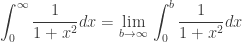
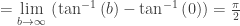


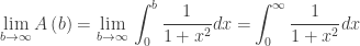
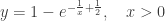
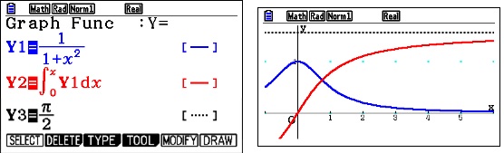 Of course, we recognize this as the inverse tangent function, but what is more interesting is that whatever this function is, it seems to have a horizontal asymptote at
 and
and  .
.


 so
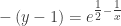
so  . Continue and solve for y.


 , which of the following values is the greatest?
 changes from positive to negative.”
  and the maximum value of
  ….” And then ask any of the questions above – some answers will be different, some will be the same. Discussing which will not change and why makes a worthwhile discussion.
 and ask the questions above. Again most of the answers will change.
  and ask the questions above. This time most of the answers will change.
 , Answer including work:
  . But I think a longer way around is also better:
 then
then  so
so  or if
or if  , then
  Solution:
  or
or  that it will be natural to say
 so
so  or if
or if  Solution:
 . Starting the same way
 so
so  which really means
 which really means
  . Then the union of these two sets looks like an intersection. The solution is
 on the other side, with > you have a union pointing away from the origin and with < you have somehow an intersection. Who needs to remember all that when this idea works all the time?
 , then
  and
and  , so
, so  and
and  or more precisely
  latex 4x-10\ge 0$, then
  and
and 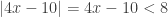 , so
, so  and
and  or more precisely
  . The union again becomes an intersection and the answer is
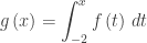
 . After separating the variables, integrating, including the “+C” and substituting the initial condition students arrived at this equation which they now need to solve for y:

 and then go ahead and solve for