L’Hôpital Rules the Graph

In my last post on May 31, 2012 I showed a way of demonstrating why L’Hôpital’s Rule works. We looked at an example,

\displaystyle \underset{x\to \pi }{\mathop{\lim }}\,\frac{\tan \left( x \right)}{\sin \left( x \right)},

which met the requirement of the theorem called L’Hôpital’s Rule, namely the functions are differentiable and, since  tan(\pi ) = sin(\pi ) = 0 they intersect on the x-axis at \left( \pi ,0 \right). We looked at the graph and then zoomed-in at \left( \pi ,0 \right).

L’Hôpital’s Rule tells us that with these conditions the limit is the same as the limit of the ratio of their slopes (or their derivatives, if you prefer). Can you see what that ratio is from Figure 2? Even though this is not a “square window” the ratio is obviously –1.

Here are four other limits. See if you can find them by the method suggested here. Namely zoom-in on the point where the functions intersect and see if you can find the limits without doing any computations. (Yes, I know you already know the first 3, but try this idea anyway. )

1. \displaystyle \underset{x\to 0}{\mathop{\lim }}\,\frac{\sin \left( x \right)}{x}

2. \displaystyle \underset{x\to 0}{\mathop{\lim }}\,\frac{1-\cos \left( x \right)}{x}

3. \displaystyle \underset{x\to 0}{\mathop{\lim }}\,\frac{\cos \left( \tfrac{\pi }{2}+x \right)}{x} also known as \displaystyle \underset{x\to 0}{\mathop{\lim }}\,\frac{\cos \left( \tfrac{\pi }{2}+x \right)-\cos \left( \tfrac{\pi }{2} \right)}{x}

4. \displaystyle \underset{x\to 1}{\mathop{\lim }}\,\frac{\pi \ln \left( x \right)}{\sin \left( \pi x \right)}


Answers in order:  1, 0, -1, -1

A Standard Problem?

Sometimes even the simplest problems can lead to interesting places. I got interested in this ordinary textbook problem a few months ago while observing an AB calculus class. Here is how my thinking went written as a series of exercises:

Original exercise: Find the point(s) on the parabola y = x2 that are closest to the point (0, 2).

The solution is straightforward:

Let z(x) be the distance from (0, 2) to the point (x, x2). Then \displaystyle z\left( x \right)=\sqrt{{{\left( x-0 \right)}^{2}}+{{\left( {{x}^{2}}-2 \right)}^{2}}}and setting the derivative equal to zero, we find the critical points at x = 0 a local maximum and x=-\sqrt{\tfrac{3}{2}} and x=\sqrt{\tfrac{3}{2}} both absolute minimums located symmetrically to the y-axis.

The students had some trouble understanding what was going on. I suggested they consider a point moving along the parabola starting high on the left side. As the point comes down the graph its distance from \left( 0,2 \right) gets shorter until it reaches some minimum length somewhere. Then the distance gets longer again until – where? Obviously, at the origin. Then symmetry takes over and the distance decreases again until it reaches a second minimum directly across the y-axis from the first point, after which it increases forever.

Exercise 1: Sketch the graph of the distance function, z(x), on top of the graph of the parabola. Give the exact coordinates of the maximum point without doing any computations. Discuss the y-coordinates of the minimum points.

It then occurred to me that there is nothing sacred about (0, 2). We could use any point on the y-axis, . Or could we? I pictured a circle centered at the point (0, a) on the y-axis tangent to the parabola (i.e. tangent to the tangent line of the parabola). The radius of such a circle is the minimum distance for that y-axis center point.

Exercise 2: If the point is below the origin then obviously the minimum distance is the distance directly up to the origin. There are places above the x-axis where the origin is the closest point. For what values of a is the origin the closest point? Use the circle mentioned above to explain how this is possible.

The distance graph that we drew above has a W shape similar to the shape of some 4th degree polynomials (note: z(x) is not a 4th degree polynomial, it is not even a polynomial). So next I drew the graph of z’(x), the first derivative of z; this graph is similar to a cubic polynomial (again it is not a polynomial)

Exercise 3: Without actually computing the derivative’s equation, sketch the graph of the derivative with the graph of the parabola and the distance function’s graph. Be sure the critical points are where they should be.

Exercise 4: Use a graphing program or a graphing calculator do draw the parabola, z(x) and z’(x) and use it to check your sketches.

Project: Using a suitable program (Winplot, Geogebra, etc.) set up an animation that will show all the features discussed above. It should show the parabola which does not move, the movable point (0, a), the circle tangent to the parabola, z(x) and z’(x). These last 3 should move with the slider for a.

At this point I noticed that the derivative changed concavity 4 times (up-down-up-down). The origin is one of 3 points of inflection. I wondered if there was anything interesting about the location of the points of inflection.

Exercise 5: Find the coordinates of the points of inflection of z’(x). Are they related to any of the features in the problem? (Use a CAS for this one.)

The solutions can be found here: Closest Point Problem Solution.

Interpreting Graphs

AP Type Questions 1

The long name is “Here’s the graph of the derivative, tell me things about the function.”

Most often students are given the graph identified as the derivative of a function. There is no equation given and it is not expected that students will write the equation (although this may be possible); rather, students are expected to determine important features of the function directly from the graph of the derivative. They may be asked for the location of extreme values, intervals where the function is increasing or decreasing, concavity, etc. They may be asked for function values at points.

The graph may be given in context and student will be asked about that context. The graph may be identified as the velocity of a moving object and questions will be asked about the motion and position. (Motion problems will be discussed as a separate type in a later post.)

Less often the function’s graph may be given and students will be asked about its derivatives.

What students should be able to do:

  • Read information about the function from the graph of the derivative. This may be approached as a derivative techniques or antiderivative techniques.
  • Find where the function is increasing or decreasing.
  • Find and justify extreme values (1st  and 2nd derivative tests, Closed interval test, aka.  Candidates’ test).
  • Find and justify points of inflection.
  • Find slopes (second derivatives, acceleration) from the graph.
  • Write an equation of a tangent line.
  • Evaluate Riemann sums from geometry of the graph only.
  • FTC: Evaluate integral from the area of regions on the graph.
  • FTC: The function, g(x), maybe defined by an integral where the given graph is the graph of  the integrand, f(t), so students should know that if,  \displaystyle g\left( x \right)=g\left( a \right)+\int_{a}^{t}{f\left( t \right)dt} then  {g}'\left( x \right)=f\left( x \right)  and  {{g}'}'\left( x \right)={f}'\left( x \right).

The ideas and concepts that can be tested with this type question are numerous. The type appears on the multiple-choice exams as well as the free-response. They have accounted for almost 25% of the points available on recent test. It is very important that students are familiar with all of the ins and outs of this situation.

As with other questions, the topics tested come from the entire year’s work, not just a single unit. In my opinion many textbooks do not do a good job with these topics.

Study past exams; look them over and see the different things that can be asked.

For some previous posts on this subject see October 151719, 24, 26, 2012 January 25, 28, 2013

Open or Closed?

About this time of year you find someone, hopefully one of your students, asking, “If I’m finding where a function is increasing, is the interval open or closed?”

Do you have an answer?

This is a good time to teach some things about definitions and theorems.

The place to start is to ask what it means for a function to be increasing. Here is the definition:

A function is increasing on an interval if, and only if, for all (any, every) pairs of numbers x1 < x2 in the interval, f(x1) < f(x2).

(For decreasing on an interval, the second inequality changes to f(x1) > f(x2). All of what follows applies to decreasing with obvious changes in the wording.)

  1. Notice that functions increase or decrease on intervals, not at individual points. We will come back to this in a minute.
  2. Numerically, this means that for every possible pair of points, the one with the larger x-value always produces a larger function value.
  3. Graphically, this means that as you move to the right along the graph, the graph is going up.
  4. Analytically, this means that we can prove the inequality in the definition.

For an example of this last point consider the function f(x) = x2. Let x2 = x1 + h where h > 0. Then in order for  f(x1) < f(x2) it must be true that

{{x}_{1}}^{2}<{{\left( {{x}_{1}}+h \right)}^{2}}
0<{{\left( {{x}_{1}}+h \right)}^{2}}-{{x}_{1}}^{2}
0<{{x}_{1}}^{2}+2h{{x}_{1}}+{{h}^{2}}-{{x}_{1}}^{2}
0<h\left( 2{{x}_{1}}+h \right)

This can only be true if {{x}_{1}}\ge 0, Thus, x2 is increasing only if x\ge 0.

Now, of course, we rarely, if ever, go to all that trouble. And it is even more trouble for a function that increases on several intervals.  The usual way of finding where a function is increasing is to look at its derivative.

Notice that the expression {{\left( {{x}_{1}}+h \right)}^{2}}-{{x}_{1}}^{2} looks a lot like the numerator of the original limit definition of the derivative of x2 at x = x1, namely \displaystyle {f}'\left( {{x}_{1}} \right)=\underset{h\to 0}{\mathop{\lim }}\,\frac{{{\left( {{x}_{1}}+h \right)}^{2}}-{{x}_{1}}^{2}}{h}. If h > 0, where the function is increasing the numerator is positive and the derivative is positive also. Turning this around we have a theorem that says, If {f}'\left( x \right)>0 for all x in an interval, then the function is increasing on the interval. That makes it much easier to find where a function is increasing: we simplify find where its derivative is positive.

There is only a slight problem in that the theorem does not say what happens if the derivative is zero somewhere on the interval. If that is the case, we must go back to the definition of increasing on an interval or use some other method. For example, the function x3 is increasing everywhere, even though its derivative at the origin is zero.

Let’s consider another example. The function sin(x) is increasing on the interval \left[ -\tfrac{\pi }{2},\tfrac{\pi }{2} \right] (among others) and decreasing on \left[ \tfrac{\pi }{2},\tfrac{3\pi }{2} \right]. It bothers some that \tfrac{\pi }{2} is in both intervals and that the derivative of the function is zero at x = \tfrac{\pi }{2}. This is not a problem. Sin(\tfrac{\pi }{2}) is larger than all the other values is both intervals, so by the definition, and not the theorem, the intervals are correct.

It is generally true that if a function is continuous on the closed interval [a,b] and increasing on the open interval (a,b) then it must be increasing on the closed interval [a,b] as well. (There is a proof by Lou Talman of this fact click here .)

Returning to the first point above: functions increase or decrease on intervals not at points. You do find questions in books and on tests that ask, “Is the function increasing at x = a.” The best answer is to humor them and answer depending on the value of the derivative at that point. Since the derivative is a limit as h approaches zero, the function must be defined on some interval around x = a in which h is approaching zero. So answer according to the value of the derivative on that interval.

You can find more on this here.

Case Closed.

Real “Real-life” Graph Reading

A few days ago, Paul Krugman wrote a blog about the job situation in the US.   Evan J. Romer, a mathematics teacher from Conklin, NY, used it as the basis for a great exercise on reading the graph of the derivative, the subject of my last post. He posted the questions to the AP Calculus Learning Community.  I liked them so much I have included them on my blog with Evan’s kind permission. The questions and solutions are here and on the Resources Tab above.

He used the graph below which shows the change in the number of non-farm jobs per month; in other words, the graph of a derivative of the number of people employed. The jagged graph is the data; the smooth graph is a model approximating the data.

The model is \displaystyle C\left( t \right)=\frac{1000{{t}^{2}}}{{{t}^{2}}+40}-800

From this Mr. Romer developed a series of questions very similar to AP questions.  Don’t overlook the last note which discusses a “classic AP calculus mistake” made by the first person to reply to Krugman’s blog.

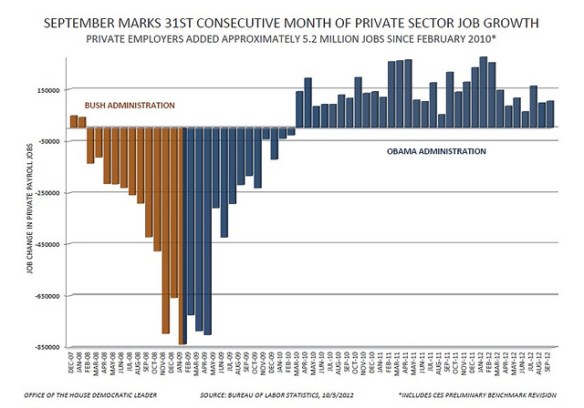
The first of Romer’s questions are integration questions, which you may not yet have gotten to with your class. Below is another graph of nearly the same data displayed as a bar graph. (Around February 2010 this was dubbed the “Bikini Graph” – if you look at the graph before that date you will see why.) It may be helpful in explaining the first of Romer’s questions to your class since each bar represents the change in the number of jobs for that month and leads into the concept of accumulation and the integral as the area between the graph and the axis. You can return to this when you introduce integration.

Thank You Evan.

Concavity

What does it mean for a graph to be concave up or down over an interval?

Not an easy question. I have seen a book where the idea was defined solely with a picture! Now pictures are good, and you should certainly use pictures to give your students a good understanding of concavity, but a definition needs a bit more. But there seems to be no general agreement on a definition.

  • My favorite definition is that a function is concave up (down) on an interval where any (every, all) line tangent to the graph in the interval lies below (above) the graph in the interval (except at the point of tangency).
  • One of the most common definitions is that if the second derivative is positive (negative) on an interval, the graph is concave up (down) on the interval.
  • Another approach is to connect any (every, all) pairs of points of the function in the interval. If all these segments (except their endpoints) lie above (below) the graph then the graph is concave up (down).
  • Yet another is that a function is concave up (down) where the first derivative is increasing (decreasing). This is not quite the same as saying a function is concave up (down) where the first derivative is positive (negative), because of the question of including or excluding the endpoints (see the post of November 2, 2012), but this too could be a definition.

The second bullet above is used to find where the graph is concave up or down. The first idea is still true and it is important to know when trying to determine whether a tangent line approximation is larger or smaller than the actual value. If the tangent line between the point of tangency and the approximated point is below the curve (that is, the curve is concave up) the approximation is an underestimate (smaller) than the actual value; if above, then an overestimate.)

A graph is concave up where its second derivative is positive and concave down where its second derivative is negative. Thus, the concavity changes where the second derivative is zero or undefined. Such a point is called a point of inflection.

The procedure for finding a point of inflection is similar to the one for finding local extreme values: (1) find where the second derivative is zero or undefined, (2) determine that the sign of the second derivative changes, and then (3) identify the point of inflection.

Finally, a pet peeve:
Back in Algebra I students learn all about the parabola y = ax2. They learn that when a is positive the graph “opens upward” or “holds water” or is a “smiley face.” Why? Why not use the correct terms – concave up and concave down – right there, right from the start?

Next: Analyzing the graph of the derivative.

Revised October 7, 2014

Extreme Values

Every function that is continuous on a closed interval must have a maximum and a minimum value on the interval. These values may all be the same (y = 2 on [-3,3]); or the function may reach these values more than once (y = sin(x)) .

The extreme values are either (1) at an endpoint of the interval (y = 4 – 2x, on [-3, 3]), or (2) at a critical number. This is known as the Extreme Value Theorem. It is a good one to “play” with: do some sketches of the different situation above; discuss why the interval must be closed.

One way the shapes can change is if the first derivative is zero or undefined at the point where two shapes join. In this case the point is a local extreme value of the function – a local maximum or minimum value. Specifically:

  • If the first derivative changes from positive to negative, the shape of the function changes from increasing to decreasing and the point is a local maximum.  If the first derivative changes from negative to positive, the shape of the function changes from decreasing to increasing and the point is a local minimum.

This is a theorem called the First Derivative Test. By finding where the first derivative changes sign and in which direction it changes (positive to negative, or negative to positive) we can locate and identify the local extreme value precisely.

  • Another way to determine if a critical number is the location of a local maximum or minimum is a theorem called the Second Derivative Test.

If the first derivative is zero (and specifically not if it is undefined) and the second derivative is positive, then the graph has a horizontal tangent line and is concave up. Therefore, this is the location of a local minimum of the function.

Likewise, if the first derivative is zero at a point and the second derivative is negative there, the function has a local maximum there.

If both the first and second derivatives are zero at a point, then the second derivative test cannot be used, for example y = x4 at the origin.

The mistake students make with the second derivative test is in not checking that the first derivative is zero.

In the case where both the first and second derivatives are zero at the same point the function changes direction but not concavity (e.g.  (x) = xat the origin), or changes concavity but not direction (e.g. .  (x) = xat the origin).

Next: More about Concavity