The fourth in the Graphing Calculator / Technology series
Comparing the graph of a function and its derivative is instructive and necessary in beginning calculus. Today I will show you how you can do this first with Desmos a free online graphing program and then on a graphing calculator. Desmos does this a lot better than graphing calculators, because of the easy use of sliders. CAS calculators also have sliders but they are not as easy to use as Desmos.
Let’s get started. Instead of presenting you with a completed Desmos graph, I will show you how to make you own. One of the things I have found over the years is that it takes some mathematical knowledge to make good demonstration graph and that in itself if useful and instructive. Hopefully, you and your students will soon be able to make your own to show exactly what you want.
Open Desmos and sign into your account; if you don’t have one then register – its free and you can keep your results and even share them with others.
In the first entry line on the left, enter the equation of the function whose graph you want to explore. Call it f(x); that is enter f(x) = your function. Later you will be able to change this to other functions and investigate them, without changing anything else.
On the second line enter the symmetric difference quotient as
Instead of a variable h, as we did in our last post in this series, enter 0.001. This will graph the derivative without having to calculate the derivative. Of course, you could enter the derivative here if your class has learned how to calculate derivatives. If so, you will have to change this line each time you change the function.
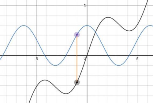
In order to closely compare the function and its derivative, on the next line enter the equation of a vertical segment from a point on the function (a, f(a)) to a point on the derivative (a, s(a)). Desmos does not have a segment operation, but here is how you graph a segment. In general, a segment from (a, b) to (c, d) is entered as the parametric/vector function

The a, b, c, and d may be numbers or functions. Since our segment is vertical the first coordinate will have a = c and will reduce to a. Here’s what to enter on the third line:

(Notice that there is no x in this expression; t is the variable. Also, the f(a) and s(a) may be interchanged.)
When you push enter, you will be prompted to add a slider for a: click to add the slider. A line will appear under the expression which will allow you to set the domain for t: click the endpoints and enter 0 on the left and 1 on the right, if necessary.
That’s it. You’re done. Use the slider to move around the graphs.
Using the graphs
Discuss with your class, or better yet divide them into groups and let them discuss, what they see. Since at this point they are probably new to this provide some hints such as “What happens on the graph of f when s is 0?” or “What is true on s when f is increasing?” or “What happens to the function at the extreme values of the derivative?” Prompt the students to look for increasing and decreasing, concavity, points of inflection, and extreme values. All the usual stuff. Work from the function to the derivative and from the derivative to the function.
Have your students formulate their results as (tentative) theorems. You actually want them to make some mistakes here, so you can help them improve their thinking and wording. For example, one result might be: If the function is increasing, then the derivative is positive. By changing the first function to an example like f(x) = x3 or f(x) = x + sin (x). Help them see that non-negative might be a better choice.
You might try giving different groups different functions and let them compare and contrast their results.
This is very much in line with MPACs 1, 2, 4, and 6.
You can do the same kind of thing with graphing calculators. That is, you can graph the function and its derivative or a difference quotient. The difference is that graphing calculators do not have sliders.
Extra feature: Desmos will graph a point if you enter the coordinates just like you write them: (a, b). The coordinates may be numbers or functions or a combination of both. Try adding two points to your graph one at each the end of the segment between the graphs that will move with the same slider.

f(x) = x + 2sin(x) and its derivative.

 Graphing and the analysis of graphs given (1) the equation, (2) a graph, or (3) a table of values of a function and its derivative(s) makes up the largest group of questions on the AP exams. Most of the other applications of the derivative depend on understanding the relationship between a function and its derivatives.
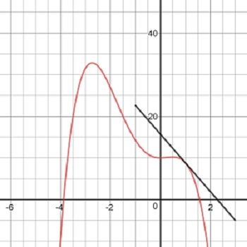

 then
then  and
and  . In this case students should write
  on their answer paper, so it is clear to the reader that they understand this.

 in the standard window. The vertical line is not really the asymptote and the “hole” at (2, 0.75) is not seen.