Reading the Derivative’s Graph

A very typical calculus problem is given the equation of a function, to find information about it (extreme values, concavity, increasing, decreasing, etc., etc.). This is usually done by computing and analyzing the first derivative and the second derivative. All the textbooks show how to do this with copious examples and exercises. I have nothing to add to that. One of the “tools” of this approach is to draw a number line and mark the information about the function and the derivative on it.

A very typical AP Calculus exam problem is given the graph of the derivative of a function, but not the equation of either the derivative or the function, to find all the same information about the function. For some reason, student find this difficult even though the two-dimensional graph of the derivative gives all the same information as the number line graph and, in fact, a lot more.

Looking at the graph of the derivative in the x,y-plane it is easy to very determine the important information. Here is a summary relating the features of the graph of the derivative with the graph of the function.

Feature the function
{y}'> 0 is increasing
{y}' < 0 is decreasing
{y}' changes  – to + has a local minimum
{y}'changes + to – has a local maximum
{y}' increasing is concave up
{y}' decreasing is concave down
{y}' extreme value has a point of inflection

Here’s a typical graph of a derivative with the first derivative features marked.

Here is the same graph with the second derivative features marked.

The AP Calculus Exams also ask students to “Justify Your Answer.” The table above, with the columns switched does that. The justifications must be related to the given derivative, so a typical justification might read, “The function has a relative maximum at x-2 because its derivative changes from positive to negative at x = -2.”

Conclusion Justification
y is increasing {y}'> 0
y is decreasing {y}'< 0
y has a local minimum {y}'changes  – to +
y has a local maximum {y}'changes + to –
y is concave up {y}'increasing
y is concave down {y}'decreasing
y has a point of inflection {y}'extreme values


For notes on vertical asymptotes see

For notes on horizontal asymptotes see Other Asymptotes

Concavity

What does it mean for a graph to be concave up or down over an interval?

Not an easy question. I have seen a book where the idea was defined solely with a picture! Now pictures are good, and you should certainly use pictures to give your students a good understanding of concavity, but a definition needs a bit more. But there seems to be no general agreement on a definition.

  • My favorite definition is that a function is concave up (down) on an interval where any (every, all) line tangent to the graph in the interval lies below (above) the graph in the interval (except at the point of tangency).
  • One of the most common definitions is that if the second derivative is positive (negative) on an interval, the graph is concave up (down) on the interval.
  • Another approach is to connect any (every, all) pairs of points of the function in the interval. If all these segments (except their endpoints) lie above (below) the graph then the graph is concave up (down).
  • Yet another is that a function is concave up (down) where the first derivative is increasing (decreasing). This is not quite the same as saying a function is concave up (down) where the first derivative is positive (negative), because of the question of including or excluding the endpoints (see the post of November 2, 2012), but this too could be a definition.

The second bullet above is used to find where the graph is concave up or down. The first idea is still true and it is important to know when trying to determine whether a tangent line approximation is larger or smaller than the actual value. If the tangent line between the point of tangency and the approximated point is below the curve (that is, the curve is concave up) the approximation is an underestimate (smaller) than the actual value; if above, then an overestimate.)

A graph is concave up where its second derivative is positive and concave down where its second derivative is negative. Thus, the concavity changes where the second derivative is zero or undefined. Such a point is called a point of inflection.

The procedure for finding a point of inflection is similar to the one for finding local extreme values: (1) find where the second derivative is zero or undefined, (2) determine that the sign of the second derivative changes, and then (3) identify the point of inflection.

Finally, a pet peeve:
Back in Algebra I students learn all about the parabola y = ax2. They learn that when a is positive the graph “opens upward” or “holds water” or is a “smiley face.” Why? Why not use the correct terms – concave up and concave down – right there, right from the start?

Next: Analyzing the graph of the derivative.

Revised October 7, 2014

Extreme Values

Every function that is continuous on a closed interval must have a maximum and a minimum value on the interval. These values may all be the same (y = 2 on [-3,3]); or the function may reach these values more than once (y = sin(x)) .

The extreme values are either (1) at an endpoint of the interval (y = 4 – 2x, on [-3, 3]), or (2) at a critical number. This is known as the Extreme Value Theorem. It is a good one to “play” with: do some sketches of the different situation above; discuss why the interval must be closed.

One way the shapes can change is if the first derivative is zero or undefined at the point where two shapes join. In this case the point is a local extreme value of the function – a local maximum or minimum value. Specifically:

  • If the first derivative changes from positive to negative, the shape of the function changes from increasing to decreasing and the point is a local maximum.  If the first derivative changes from negative to positive, the shape of the function changes from decreasing to increasing and the point is a local minimum.

This is a theorem called the First Derivative Test. By finding where the first derivative changes sign and in which direction it changes (positive to negative, or negative to positive) we can locate and identify the local extreme value precisely.

  • Another way to determine if a critical number is the location of a local maximum or minimum is a theorem called the Second Derivative Test.

If the first derivative is zero (and specifically not if it is undefined) and the second derivative is positive, then the graph has a horizontal tangent line and is concave up. Therefore, this is the location of a local minimum of the function.

Likewise, if the first derivative is zero at a point and the second derivative is negative there, the function has a local maximum there.

If both the first and second derivatives are zero at a point, then the second derivative test cannot be used, for example y = x4 at the origin.

The mistake students make with the second derivative test is in not checking that the first derivative is zero.

In the case where both the first and second derivatives are zero at the same point the function changes direction but not concavity (e.g.  (x) = xat the origin), or changes concavity but not direction (e.g. .  (x) = xat the origin).

Next: More about Concavity

Joining the Pieces of a Graph

In this post we will consider how the shapes discussed in the previous two posts can join together. Continuity and the derivative at the point where two shapes join tell us what’s going on.

Graphs can change from one shape to another only at places where:

  • The first derivative changes sign. For this to happen, the first derivative has to be either zero or undefined.  The x-coordinate at such places is called a critical number; the point is called a critical point. The function may have a local extreme value (a maximum or minimum) at its critical values. Not all critical numbers are the location of an extreme value, but all extreme values occur at critical numbers.
  • The second derivative changes sign. Such places are called a point of inflection (or, outside of the USA, point of inflexion.)  As with the first derivative, the second derivative can change sign only where it is zero or undefined. (Also, in order for there to be a second derivative at a point, the first derivative cannot be undefined there.)
  • The function is not continuous. The separate pieces can easily be different shapes. This really falls under the first bullet above, but functions may be continuous and still fail to have a derivative at a critical number.

This suggests a procedure: First, find the critical numbers by finding where {f}'\left( x \right)=0 or is undefined and then determining if there is a change of sign of the first derivative at the critical number. This may be the location of an extreme value. Compare y = x2 and y = x3 at the origin.

Do the same for points of inflection: find where {{f}'}'\left( x \right)=0 or is undefined and determine if there is a sign change there. These places may be points of inflection. Compare y = x3 and y = x4 at the origin.

A word of caution: Some authors require a non-vertical tangent line at a point of inflection and/or that the derivative exists there. This eliminates functions like y = x1/3 which has no derivative at the origin and a vertical tangent line. I see no reason for this: if there is a point where the concavity changes, that’s a point of inflection. Still you should go with your textbook’s author. The AP exams avoid asking about this situation.

If the function is not continuous (and therefore not differentiable) at a point, then the shapes don’t join. You need to look separately on each side of the point where the function is not continuous. The missing point, the jump or step, or the vertical asymptote is the clue that there may be a change in the shape. There does not have to be a change in shape at all, but as with all discontinuities be sure to check what’s happening on both sides. .

If the function is continuous, but not differentiable at a point then the shape may, but does not have to change shape there. If this is the case, the graph is not locally linear. It may have a sharp point or just a little “kink” there. But the non-differentiability tells us that something interesting is happening there.

Next: Extreme Values

The Shapes of a Graph

In my last post we discussed the five shapes of a graph. Hopefully, that activity, which is posted under the Resources tab above, helped your students discover that

  • A function is increasing and concave up, on any interval where its first derivative is positive and its second derivative is positive, like y = sin(x) on \left( \tfrac{3\pi }{2},2\pi \right).
  • A function is increasing and concave down, on any interval were its first derivative is positive and its second derivative is negative, like y = sin(x) on  \left( 0,\tfrac{\pi }{2} \right).
  • A function is decreasing and concave up, on any interval where its first derivative is negative and its second derivative is positive, like y = sin(x) on \left( \pi ,\tfrac{3\pi }{2} \right).
  • A function is decreasing and concave down, on any interval where its first derivative is negative and its second derivative is negative, like y = sin(x) on \left( \tfrac{\pi }{2},\pi \right).
  • To which we will add a function is linear where its first derivative is constant and its second derivative is zero.

Separating the increasing/decreasing behavior from the concavity:

  • On an interval where the first derivative is positive the graph is increasing, and on an interval where the first derivative is negative the function is decreasing.
  • On an interval where the second derivative is positive the function is concave, on an interval where the second derivative is negative the graph is concave down.

Be careful when presenting the ideas above.

None of them consider what happens if one of the other of the derivatives is zero or undefined. There is an important theorem which says, and we must be careful here, “If for all x in an interval, {f}'\left( x \right)>0 , then the function is increasing on that interval.”

True enough, but what about y = x3 on an interval containing the origin? Well, the theorem does not apply, since the derivative is not positive everywhere on the interval. The theorem says nothing about what happens when the derivative is zero, only what happens when it is positive.  In such cases we need to return to the definition of increasing (which incidentally does not mention derivatives), to determine that y = x3 is increasing on any interval containing the origin (any interval, anywhere, in fact).

Another thing to be careful of is this: Functions increase or decrease on intervals, not at points. If you are asked if a function is increasing or decreasing at a point, or “Is the velocity increasing when t = ….” interpret the question as asking, “Is there a small open interval containing the point, on which the function is increasing or decreasing.”

Using the derivative to give this kind of information about the graph is a big part of the calculus and one of the important uses of derivatives. We can determine information by working with the equation of the derivative. We can also work from the graph of the derivative. This is often easier since it is easy to tell from the graph when the derivative is positive or negative. From the graph of the derivative, we can also see where the derivative is increasing or decreasing, and this tells us the sign of the second derivative and hence about the concavity of the function. I will discuss this in a later post.

Next: Joining the Pieces

Concepts Related to Graphs

This and the next several posts will be about graphing and specifically how the function and its first and second derivatives are related. Since I do not intend this to be a textbook, I will not be doing textbook stuff. Rather, I hope to add some big picture things about the concepts involved. Hope you find it useful.

________________________________

Graphs of functions come in some combination of five shapes:

• Linear,
• Increasing, concave up,
• Increasing, concave down,
• Decreasing, concave up, and
• Decreasing, concave down.

I have put together an activity, An Exploration of the Shape of a Graph, to help students learn the relationship between the shapes and the derivative. Leaving the linear sections aside, the idea of the activity is to call students’ attention to the other four shapes and the slope of the tangent line (the derivative) in the intervals where the graph has each shape.

The key is to keep focused on the tangent line. To this end I suggest drawing short tangent segments parallel to the graph, as illustrated in the figure below.

Air-graphing: Another way to help students internalize this idea is to draw the graph of a function on the board and then have the students hold their pen out in front of them so the pen looks like a segment tangent to the graph. Then move the pen along the graph paying attention to the slope.

Either way what you want students to be aware of is

(1) Where the slopes are positive and where they are negative. This will later be related to the intervals where the function increases and decreases, and

(2) How the slope itself is changing. Is the slope increasing or decreasing? This will later be related to the concavity.

I hope you and your students find this activity helpful.

Why Radians?

Calculus is always done in radian measure. Degree (a right angle is 90 degrees) and gradian measure (a right angle is 100 grads) have their uses. Outside of the calculus they may be easier to use than radians. However, they are somewhat arbitrary. Why 90 or 100 for a right angle? Why not 10 or 217?

Radians make it possible to relate a linear measure and an angle measure. A unit circle is a circle whose radius is one unit. The one-unit radius is the same as one unit along the circumference. Wrap a number line counterclockwise around a unit circle starting with zero at (1, 0). The length of the arc subtended by the central angle becomes the radian measure of the angle.

This keeps all the important numbers like the sine and cosine of the central angle, on the same scale. When you graph y = sin(x) one unit in the x-direction is the same as one unit in the y-direction. When graphing using degrees, the vertical scale must be stretched a lot to even see that the graph goes up and down. Try graphing on a calculator y = sin(x) in degree mode in a square window and you will see what I mean.

But the utility of radian measure is even more obvious in calculus. To develop the derivative of the sine function you first work with this inequality (At the request of a reader I have added an explanation of this inequality at the end of the post):

\displaystyle \frac{1}{2}\cos \left( \theta \right)\sin \left( \theta \right)\le \frac{1}{2}\theta \le \frac{1}{2}\tan \left( \theta \right)

From this inequality you determine that \displaystyle \underset{\theta \to 0}{\mathop{\lim }}\,\frac{\sin \left( \theta \right)}{\theta }=1

The middle term of the inequality is the area of a sector of a unit circle with central angles of \theta 
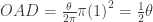
radians. If you work in degrees, this sector’s area is \displaystyle \frac{\pi }{360}\theta  and you will find that
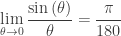
 \displaystyle \underset{\theta \to 0}{\mathop{\lim }}\,\frac{\sin \left( \theta \right)}{\theta }=\frac{\pi }{180}.

This limit is used to find the derivative of the sin(x). Thus, with x in degrees, \displaystyle \frac{d}{dx}\sin \left( x \right)=\frac{\pi }{180}\cos \left( x \right)
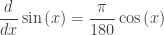
. This means that with the derivative or antiderivative of any trigonometric function that \displaystyle \frac{\pi }{180} is there getting in the way.

Who needs that?

Do your calculus in radians.


Revision December 7, 2014: The inequality above is derived this way. Consider the unit circle shown below.

unit circle

1. The central angle is \theta  and the coordinates of A are \left( \cos (\theta ),\sin (\theta ) \right).

Then the area of triangle OAB is \frac{1}{2}\cos \left( \theta\right)\sin \left( \theta\right)

2. The area of sector OAD=\frac{\theta}{2\pi }\pi {{\left( 1 \right)}^{2}}=\frac{1}{2}\theta 
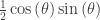
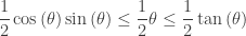
. The sector’s area is larger than the area of triangle OAB.
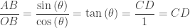
3. By similar triangles \displaystyle \frac{AB}{OB}=\frac{\sin \left( \theta\right)}{\cos \left( \theta\right)}=\tan \left( \theta\right)=\frac{CD}{1}=CD.

Then the area of \Delta OCD=\frac{1}{2}CD\cdot OD=\frac{1}{2}\tan \left( \theta \right) This is larger than the area of the sector, which establishes the inequality above.

Multiply the inequality by \displaystyle \frac{2}{\sin \left( \theta \right)} and take the reciprocal to obtain
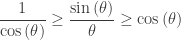
 \displaystyle \frac{1}{\cos \left( \theta \right)}\ge \frac{\sin \left( \theta \right)}{\theta }\ge \cos \left( \theta \right).

Finally, take the limit of these expression as \theta \to 0 and the limit \displaystyle \underset{\theta \to 0}{\mathop{\lim }}\,\frac{\sin \left( \theta \right)}{\theta }=1 is established by the squeeze theorem.