
This is the first of a series of blog posts that I plan to write over the next few months, staying a little ahead of where you are so you can use anything you find useful in your planning. Look for this series every 2 – 4 weeks.
Unit 1 contains topics on Limits and Continuity. (CED – 2019 p. 36 – 50). These topics account for about 10 – 12% of questions on the AB exam and 4 – 7% of the BC questions.
Logically, limits come before continuity since limit is used to define continuity. Practically and historically, continuity comes first. Newton and Leibnitz did not have the concept of limit the way we use it today. It was in the early 1800’s that the epsilon-delta definition of limit was first given by Bolzano (whose work was overlooked) and then by Cauchy and Weierstrass. But their formulation did not use the word “limit”, rather the use was part of their definition of continuity. Only later was it pulled out as a separate concept and then returned to the definition of continuity as a previously defined term.
Students should have plenty of experience in their math courses before calculus with functions that are and are not continuous. They should know the names of the types of discontinuities – jump, removable, infinite, etc. As you go through this unit, you may want to quickly review these terms and concepts as they come up.
(As a general technique, rather than starting the year with a week or three of review – which the students need but will immediately forget again – be ready to review topics as they come up during the year as they are needed – you will have to do that anyway. See Getting Started #2)
Topics 1.1 – 1.9: Limits
Topic 1.1: Suggests an introduction to calculus to give students a hint of what’s coming. See Getting Started #3
Topic 21.: Proper notation and multiple-representations of limits.
There is an exclusion statement noting that the delta-epsilon definition of limit is not tested on the exams, but you may include it if you wish. The epsilon-delta definition is not tested probably because it is too difficult to write good questions. Specifically, (1) the relationship for a linear function is always 
Topic 1.3: One-sided limits.
Topic 1.4: Estimating limits numerically and from tables.
Topic 1.5: Algebraic properties of limits.
Topic 1.6: Simplifying expressions to find their limits. This can and should be done along with learning the other concepts and procedures in this unit.
Topic 1.7: Selecting the proper procedure for finding a limit. The first step is always to substitute the value into the limit. If this comes out to be number than that is the limit. If not, then some manipulation may be required. This can and should be done along with learning the other concepts and procedures in this unit.
Topic 1.8: The Squeeze Theorem is mainly used to determine 
Topic 1.9: Connecting multiple-representations of limit. This can and should be done along with learning the other concepts and procedures in this unit. Dominance, Topic 15, may be included here as well (EK LIM-2.D.5)
Topics 1.10 – 1.16 Continuity
Topic 1.10: Here you can review the different types of discontinuities with examples and graphs.
Topic 1.11: The definition of continuity. The EK statement does not seem to use the three-hypotheses definition. However, for the limit to exist and for f(c) to exist, they must be real numbers (i.e. not infinite). This is tested often on the exams, so students should have practice with verifying that (all three parts of) the hypothesis are met and including this in their answers.
Topic 1.12: Continuity on an interval and which Elementary Functions are continuous for all real numbers.
Topic 1.13: Removable discontinuities and handing piecewise – defined functions
Topic 1.14: Vertical asymptotes and unbounded functions. Here be sure to explain the difference between limits “equal to infinity” and limits that do not exist (DNE). See Good Question 5: 1998 AB2/BC2.
Topic 1.15: Limits at infinity, or end behavior of a function. Horizontal asymptotes are the graphical manifestation of limits at infinity or negative infinity. Dominance is included here as well (EK LIM-2.D.5)
Topic 1.16: The Intermediate Value Theorem (IVT) is a major and important result of a function being continuous. This is perhaps the first Existence Theorem students encounter, so be sure to stop and explain what an existence theorem is.
The suggested number of 40 – 50 minute class periods is 22 – 23 for AB and 13 – 14 for BC. This includes time for testing etc. If time seems to be a problem you can probably combine topics 3 – 5, topics 6 -7, topics 11 – 12. Topics 6, 7, and 9 are used with all the limit work.
There are three other important limits that will be coming in later Units:
The definition of the derivative in Unit 2, topics 1 and 2
L’Hospital’s Rule in Unit 4, topic 7
The definition of the definite integral in Unit 6, topic 3.
Posts on Continuity
CONTINUITY To help understand limits it is a good idea to look at functions that are not continuous. Historically and practically, continuity should come before limits. On the other hand, the definition of continuity requires knowing about limits. So, I list continuity first. The modern definition of limit was part of Weierstrass’ definition of continuity.
Continuity (8-13-2012)
Continuity (8-21-2013) The definition of continuity.
Continuous Fun (10-13-2015) A fuller discussion of continuity and its definition
Right Answer – Wrong Question (9-4-2013) Is a function continuous even if it has a vertical asymptote?
Asymptotes (8-15-2012) The graphical manifestation of certain limits
Fun with Continuity (8-17-2012) the Diriclet function
Far Out! (10-31-2012) When the graph and dominance “disagree” From the Good Question series
Posts on Limits
Why Limits? (8-1-2012)
Deltas and Epsilons (8-3-2012) Why this topic is not tested on the AP Calculus Exams.
Finding Limits (8-4-2012) How to…
Dominance (8-8-2012) See limits at infinity
Determining the Indeterminate (12-6-2015) Investigating an indeterminate form from a differential equation. From the Good Question series.
Locally Linear L’Hôpital (5-31-2013) Demonstrating L’Hôpital’s Rule (a/k/a L’Hospital’s Rule)
L’Hôpital’s Rules the Graph (6-5-2013)
Here are links to the full list of posts discussing the ten units in the 2019 Course and Exam Description.
2019 CED – Unit 1: Limits and Continuity
2019 CED – Unit 2: Differentiation: Definition and Fundamental Properties.
2019 CED – Unit 3: Differentiation: Composite , Implicit, and Inverse Functions
2019 CED – Unit 4 Contextual Applications of the Derivative Consider teaching Unit 5 before Unit 4
2019 – CED Unit 5 Analytical Applications of Differentiation Consider teaching Unit 5 before Unit 4
2019 – CED Unit 6 Integration and Accumulation of Change
2019 – CED Unit 7 Differential Equations Consider teaching after Unit 8
2019 – CED Unit 8 Applications of Integration Consider teaching after Unit 6, before Unit 7
2019 – CED Unit 9 Parametric Equations, Polar Coordinates, and Vector-Values Functions
2019 CED Unit 10 Infinite Sequences and Series
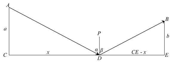
 and
and  are all perpendicular to
  the total distance is AD + DB. Therefore:
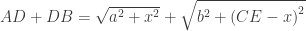


 and
and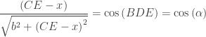
 QED.
QED.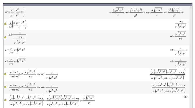
 with a > b > 0. Solving for y there are two equations, the second one is for the upper half that we will use below. The other for the lower half.
 and
and  .
. to avoid working with an undefined slope. The focus is at
  .
.

 . Don’t tell them this – drag it out of them if necessary.) Why? How do you know this?

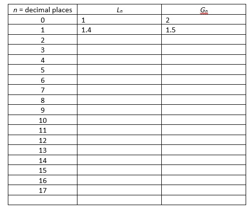
 is read, “n approaches infinity,” that infinity,
  , is not a number. The symbol
  where
where  is one of the digits 0, 1, 2, 3, …, 9, but there is no formula for listing the values of
  which converges to
  . Therefore,
 . Find this number the usual way (simplify and use long division) and compare the results.
 . Find this number the usual way and compare the results.
 .
. .
. .
. .
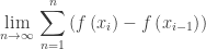
. resembles the right side of the Mean Value Theorem above. Since all the conditions are met, the MVT tells us that in each subinterval
 ![\displaystyle [{{x}_{{i-1}}},{{x}_{i}}]](https://s0.wp.com/latex.php?latex=%5Cdisplaystyle+%5B%7B%7Bx%7D_%7B%7Bi-1%7D%7D%7D%2C%7B%7Bx%7D_%7Bi%7D%7D%5D&bg=ffffff&fg=333333&s=0&c=20201002) there exists a number, call it ci , such that
there exists a number, call it ci , such that and therefore
 – The Fundamental Theorem of Calculus.)
 for all x in the interval. Every function continuous on a closed interval
  for all x in the interval. Every function continuous on a closed interval
  changes sign in the interval, then
  .
.
 is called the remainder. The equation above says that if you can find the correct c the function is exactly equal to Tn(x) + R. Notice the form of the remainder is the same as the other terms, except it is evaluated at the mysterious c. The trouble is we almost never can find the c without knowing the exact value of f(x), but; if we knew that, there would be no need to approximate. However, often without knowing the exact values of c, we can still approximate the value of the remainder and thereby, know how close the polynomial Tn(x) approximates the value of f(x) for values in x in the interval, i. See
  and their multiples.