2019 CED Unit 7: Differential Equations

Applications (Unit 8) seem to fit more logically after the opening unit on integration (Unit 6). The Course and Exam Description (CED) present differential equations first probably because the previous unit ended with techniques of antidifferentiation. My guess is that many teachers will teach Unit 8: Applications of Integration before Unit 7: Differential Equations. Therefore, for those who want to present unit 8 first, I will post unit 8 next week on December 3, 2019. That way you’ll have both for reference and can choose the order you think will work best for your students. 

Unit 7 is an introduction to the initial ideas and easy techniques related to differential equations. (CED – 2019 p. 129 – 142). These topics account for about 6 – 12% of questions on the AB exam and 6 – 9% of the BC questions.

Topics 7.1 – 7.9

Topic 7.1 Modeling Situations with Differential Equations Relating a function and its derivatives.

Topic 7.2 Verifying Solutions for Differential Equations A proposed solution to a differential equation can be checked by substituting the function and its derivative(s) into the original differential equation. There may be an infinite number of general solutions (solutions with one or more constants).

Topic 7.3 Sketching Slope Fields Slope fields are a graphical representation of a differential equation and provide information about the behavior of the solutions.

Topic 7.4 Reasoning Using Slope Fields 

Topic 7.5 Approximating Solutions Using Euler’s method (BC ONLY) A numerical approach to approximating solutions of a differential equation.

Topic 7.6 Finding General Solutions Using Separation of Variable Since this unit is only an introduction to differential equations, the method of separation of variable is the only solution method tested on the AB and BC exams.

Topic 7.7 Finding Particular Solutions Using Initial Conditions and Separation of Variables An initial condition (i.e. a point on the particular solution) allows you to evaluate the constant in the general solution and find the one solution that contains the initial condition. Also, if \displaystyle \frac{{dy}}{{dx}}=f\left( x \right) has the initial condition \displaystyle \left( {a,F\left( a \right)} \right), then the solution is \displaystyle F\left( x \right)=F\left( a \right)+\int_{a}^{x}{{f\left( x \right)dx}}. Solution may also be subject to domain restrictions

Topic 7.8 Exponential Models with Differential Equations Applications include linear motion and exponential growth and decay. The growth and decay model is \displaystyle \frac{{dy}}{{dt}}=ky with the initial condition\displaystyle (0,{{y}_{0}}) has the solution \displaystyle y={{y}_{0}}{{e}^{{kt}}}.

Topic 7.9 Logistic Models with Differential Equations (BC ONLY) The model of logistic growth, \displaystyle \frac{{dy}}{{dt}}=ky\left( {a-y} \right), can be solved by separating the variables and using partial fraction decomposition. This has never been tested (probably because solving requires a large amount of complicated algebra). Students are expected to know how to interpret the properties of the solution directly from the differential equation (asymptotes, carrying capacity, point where changing the fastest, etc.) and discuss what they mean in context without actually solving the equation.


Timing

The suggested time for Unit 7 is  8 – 9 classes for AB and 9 – 10 for BC of 40 – 50-minute class periods, this includes time for testing etc.


Previous posts on these topics for both AB and BC include:

Differential Equations A summary of the terms and techniques about differential equations and the method of separation of variables

Domain of a Differential Equation – On domain restrictions.

Accumulation and Differential Equations 

Slope Fields

An Exploration in Differential Equations An exploration illustrating many of the ideas of differential equations. The exploration is here in PDF form and the solution is here. The ideas include: finding the general solution of the differential equation by separating the variables, checking the solution by substitution, using a graphing utility to explore the solutions for all values of the constant of integration, finding the solutions’ horizontal and vertical asymptotes, finding several particular solutions, finding the domains of the particular solutions, finding the extreme value of all solutions in terms of C, finding the second derivative (implicit differentiation), considering concavity, and investigating a special case or two. 

Posts on BC Only Topics

Euler’s Method

Euler’s Method for Making Money

The Logistic Equation 

Logistic Growth – Real and Simulated


Here are links to the full list of posts discussing the ten units in the 2019 Course and Exam Description.

2019 CED – Unit 1: Limits and Continuity

2019 CED – Unit 2: Differentiation: Definition and Fundamental Properties.

2019 CED – Unit 3: Differentiation: Composite , Implicit, and Inverse Functions

2019 CED – Unit 4 Contextual Applications of the Derivative  Consider teaching Unit 5 before Unit 4

2019 – CED Unit 5 Analytical Applications of Differentiation  Consider teaching Unit 5 before Unit 4

2019 – CED Unit 6 Integration and Accumulation of Change

2019 – CED Unit 7 Differential Equations  Consider teaching after Unit 8

2019 – CED Unit 8 Applications of Integration   Consider teaching after Unit 6, before Unit 7

2019 – CED Unit 9 Parametric Equations, Polar Coordinates, and Vector-Values Functions 

2019 CED Unit 10 Infinite Sequences and Series


π from Collisions

One of my sons sent me the link to the videos below. They show a very unusual way to find the digits of π. The problems and its two solutions show the connections and the interplay between mathematics and physics. The quality of the illustrations and the verbal explanations are excellent.

Here are the main concepts used in solving the problem:

From physics:

  • Conservation of energy,
  • Conservation of momentum,
  • Phase space,
  • Phase diagram,
  • Optics (angle of incidence equals angle of reflection),
  • Dot product and column vectors.

From high school math:

  • Geometry (the inscribed angle theorem),
  • Simultaneous equations,
  • Analytic geometry,
  • Equation of a line and translations,
  • Equation of a circle.

From calculus:

  • power series for the Inverse Tangent function,
  • related rates,
  • error analysis (not the Lagrange or alternating series error bounds),
  • slope in parametric form dy/dt, and dx/dt.

Here are the videos. (The second should open after the first, and the third after the second; or, you may click on one at a time.)

The most unexpected answer to a counting puzzle (5:12)

So why do colliding blocks compute pi? (15.15)

How colliding blocks act like a beam of light … to compute pi  (14:40)


The videos are on the YouTube site 3blue1brown, by Grant Sanderson. The site describes itself as some combination of math and entertainment, depending on your disposition. The goal is for explanations to be driven by animations and for difficult problems to be made simple with changes in perspective.

The site contains a number of other videos that look like they are worth watching.


2019 CED Unit 6: Integration and Accumulation of Change

Unit 6 develops the ideas behind integration, the Fundamental Theorem of Calculus, and Accumulation. (CED – 2019 p. 109 – 128 ). These topics account for about 17 – 20% of questions on the AB exam and 17 – 20% of the BC questions.

Topics 6.1 – 6.4 Working up to the FTC

Topic 6.1 Exploring Accumulations of Change Accumulation is introduced through finding the area between the graph of a function and the x-axis. Positive and negative rates of change, unit analysis.

Topic 6.2 Approximating Areas with Riemann Sums Left-, right-, midpoint Riemann sums, and Trapezoidal sums, with uniform partitions are developed. Approximating with numerical methods, including use of technology are considered. Determining if the approximation is an over- or under-approximation.

Topic 6.3 Riemann Sums, Summation Notation and the Definite Integral. The definition integral is defined as the limit of a Riemann sum.

Topic 6.4 The Fundamental Theorem of Calculus (FTC) and Accumulation Functions Functions defined by definite integrals and the FTC.

Topic 6.5 Interpreting the Behavior of Accumulation Functions Involving Area Graphical, numerical, analytical, and verbal representations.

Topic 6.6 Applying Properties of Definite Integrals Using the properties to ease evaluation, evaluating by geometry and dealing with discontinuities.

Topic 6.7 The Fundamental Theorem of Calculus and Definite Integrals Antiderivatives. (Note: I suggest writing the FTC in this form \displaystyle \int_{a}^{b}{{{f}'\left( x \right)}}dx=f\left( b \right)-f\left( a \right) because it seems more efficient than using upper case and lower-case f.)

Topics 6.5 – 6.14 Techniques of Integration

Topic 6.8 Finding Antiderivatives and Indefinite Integrals: Basic Rules and Notation. Using basic differentiation formulas to find antiderivatives. Some functions do not have closed-form antiderivatives. (Note: While textbooks often consider antidifferentiation before any work with integration, this seems like the place to introduce them. After learning the FTC students have a reason to find antiderivatives. See Integration Itinerary

Topic 6.9 Integration Using Substitution The u-substitution method. Changing the limits of integration when substituting.

Topic 6.10 Integrating Functions Using Long Division and Completing the Square 

Topic 6.11 Integrating Using Integration by Parts (BC ONLY)

Topic 6.12 Integrating Using Linear Partial Fractions (BC ONLY)

Topic 6.13 Evaluating Improper Integrals (BC ONLY) Showing the work requires students to show correct limit notation.

Topic 6.14 Selecting Techniques for Antidifferentiation This means practice, practice, practice.


Timing

The suggested time for Unit 6 is  18 – 20 classes for AB and 15 – 16 for BC of 40 – 50-minute class periods, this includes time for testing etc.


Previous posts on these topics include:

Introducing the Derivative

Integration Itinerary

The Old Pump and Flying to Integrationland   Two introductory explorations

Working Towards Riemann Sums

Riemann Sums

The Definition of the Definite Integral

Foreshadowing the FTC 

The Fundamental Theorem of Calculus

More About the FTC

Y the FTC?

Area Between Curves

Under is a Long Way Down 

Properties of Integrals 

Trapezoids – Ancient and Modern  On Trapezoid sums

Good Question 9 – Riemann Reversed   Given a Riemann sum can you find the Integral it converges to?  A common and difficult AP Exam problem

Accumulation

Accumulation: Need an Amount?

Good Question 7 – 2009 AB 3

Good Question 8 – or Not?  Unit analysis

AP Exams Accumulation Question    A summary of accumulation ideas.

Graphing with Accumulation 1

Graphing with Accumulation 2

Accumulation and Differential Equations 

Painting a Point

Techniques of Integrations (AB and BC)

Antidifferentiation

Why Muss with the “+C”?

Good Question 13  More than one way to skin a cat.

Integration by Parts – a BC Topic

Integration by Parts 1

Integration by Part 2

Parts and More Parts

Good Question 12 – Parts with a Constant?

Modified Tabular Integration 

Improper Integrals and Proper Areas

Math vs the Real World Why \displaystyle \int_{{-\infty }}^{\infty }{{\frac{1}{x}}}dx does not converge.


Here are links to the full list of posts discussing the ten units in the 2019 Course and Exam Description.

2019 CED – Unit 1: Limits and Continuity

2019 CED – Unit 2: Differentiation: Definition and Fundamental Properties.

2019 CED – Unit 3: Differentiation: Composite , Implicit, and Inverse Functions

2019 CED – Unit 4 Contextual Applications of the Derivative  Consider teaching Unit 5 before Unit 4

2019 – CED Unit 5 Analytical Applications of Differentiation  Consider teaching Unit 5 before Unit 4

2019 – CED Unit 6 Integration and Accumulation of Change

2019 – CED Unit 7 Differential Equations  Consider teaching after Unit 8

2019 – CED Unit 8 Applications of Integration   Consider teaching after Unit 6, before Unit 7

2019 – CED Unit 9 Parametric Equations, Polar Coordinates, and Vector-Values Functions 

2019 CED Unit 10 Infinite Sequences and Series


Asymptotes and the Derivative

What does an asymptote of the derivative tell you about the function? How do asymptotes of a function appear in the graph of the derivative?

One of my most read posts is Reading the Derivative’s Graph, first published seven years ago. The long title is “Here’s the graph of the derivative; tell me about the function.” It tells how to quickly find information about the graph of a function from the derivative’s graph. I received a question from a reader recently that asked about asymptotes and the derivative, a topic that I did not cover in that post. So, I tried to find the relationship. The short answer is that an asymptote of the derivatives does not tell you much about the graph of the function. (This is probably why the idea has never been tested on the AP Calculus Exams.)

Nevertheless, there is some calculus to be learned here. You may be able to find some questions for your students to investigate on this topic. Here’s what i determined.

Before we start, here are two terms that are useful, but not commonly used.

  • An even vertical asymptote is one for which the function increases or decreases without limit on both sides of the asymptote. In other words, as x approaches a the function approaches infinity or negative infinity from both sides. The function f\left( x \right)=\frac{1}{{{{{\left( {x-2} \right)}}^{2}}}} 
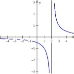
has an even vertical asymptote at x = 2. (Figure 1)
  • An odd vertical asymptote is one for which the function increases without bound on one side and decreases without bound on the other. The function g\left( x \right)=\frac{1}{{x-2}} has an odd vertical asymptote at x = 2. (Figure 2) Likewise, the tangent, cotangent, secant, and cosecant functions have odd vertical asymptotes.
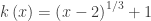
If a function has an odd vertical asymptote, then its derivative will have an even vertical asymptote. (Ask your students to explain why.)

If a function has an even vertical asymptote, then its derivative will have an odd vertical asymptote. (Ask your students to explain why.)

The converses of these two statements are false. That is, a vertical asymptote of the derivative does not necessarily indicate an asymptote of the function. The catch is continuity.

Continuous Functions

If the derivative exists at xa, then the function is continuous there. But, since we are considering asymptotes of the derivative, we cannot know from the derivative alone if the function is continuous where the derivative has an asymptote.

A simple cusp is a situation in which at an extreme point the graph is tangent to a vertical line. See Figure 3. (Or, you could say, the tangent lines from each side are coincident. Here we will limit the discussion to a vertical tangent line.) A continuous function that has a cusp will show an odd vertical asymptote on its derivative’s graph. 

An example is\displaystyle h\left( x \right)=\sqrt[3]{{{{{\left( {x-2} \right)}}^{2}}}}+1  that has a cusp at the point (2,1). (Figure 3).

A continuous function that has a vertical tangent line not a cusp, has an even vertical asymptote on its derivative’s graph. For example, k\left( x \right)={{\left( {x-2} \right)}^{{1/3}}}+1 
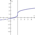
at (2,0) (Figure 4).

If you are given the graph of the derivative and it shows a vertical asymptote at x = a, and you know the function is continuous there, then

  • an odd vertical asymptote of the derivative indicates cusp on the graph of the function. This will also be an extreme value. (Ask your students to explain why.)
  • an even vertical asymptote of the derivative indicates vertical tangent line on the graph of the function, but not an extreme value. (Ask your students to explain why.)

Other than these, there is no easy way to tell what situation produced an asymptote on the derivative.

Functions that are not continuous

If the function is not continuous at xa, then things get a lot more complicated.

  • If the function is not continuous at x = a, then an even vertical asymptote of the derivative may indicate an odd vertical asymptote on the graph of the function. There is no way to be sure.
  • If the function is not continuous at x = a, then an odd vertical asymptote of the derivative may indicate an even vertical asymptote on the graph of the function. There is no way to be sure.

Consider this function: \displaystyle z\left( x \right)=\left\{ {\begin{array}{*{20}{c}} {\sqrt[3]{{{{{\left( {x-2} \right)}}^{2}}}}-1} & {x<2} \\ {\sqrt[3]{{{{{\left( {x-2} \right)}}^{2}}}}+1} & {x\ge 2} \end{array}} \right.

See Figure 5. The function is defined for all Real numbers and has a jump discontinuity at x = 2. The derivative has an odd vertical asymptote there: \displaystyle \underset{{x\to 2-}}{\mathop{{\lim }}}\,{z}'\left( x \right)=-\infty and \displaystyle \underset{{x\to 2+}}{\mathop{{\lim }}}\,{z}'\left( x \right)=-\infty . Compare this with h(x) above.

In fact,\displaystyle {h}'\left( x \right)={z}'\left( x \right)=\tfrac{2}{3}{{\left( {x-2} \right)}^{{-1/3}}},x\ne 2. Go figure.

For considerations of horizontal asymptotes and the derivative see Other Asymptotes