Given equations that define a region in the plane students are asked to find its area and the volume of the solid formed when the region is revolved around a line or used as a base of a solid with regular cross-sections. This standard application of the integral has appeared every year since 1969 on the AB exam and all but one year on the BC exam.
What students should be able to do:
- Find the intersection(s) of the graphs and use them as limits of integration (calculator equation solving). Write the equation followed by the solution; showing work is not required. Usually no credit is earned until the solution is used in context (as a limit of integration). Students should know how to store and recall these values to save time and avoid copy errors.
- Find the area of the region between the graph and the x-axis or between two graphs.
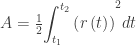
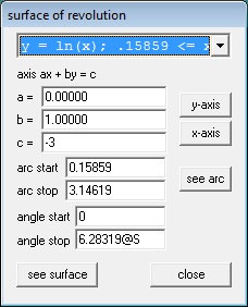
- Find the volume when the region is revolved around a line, not necessarily an axis or an edge of the region, by the disk/washer method.
- The cylindrical shell method will never be necessary for a question on the AP exams, but is eligible for full credit if properly used.
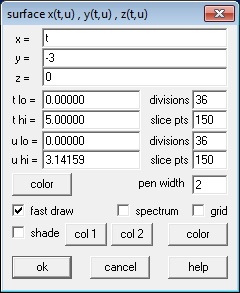
- Find the volume of a solid with regular cross-sections whose base is the region between the curves. For an interesting variation on this idea see 2009 AB 4(b)
- Find the equation of a vertical line that divides the region in half (area or volume). This involves setting up and solving an integral equation where the limit is the variable for which the equation is solved.
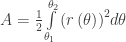
- For BC only – find the area of a region bounded by polar curves:
If this question appears on the calculator active section, it is expected that the definite integrals will be evaluated on a calculator. Students should write the definite integral with limits on their paper and put its value after it. It is not required to give the antiderivative and if a student gives an incorrect antiderivative they will lose credit even if the final answer is (somehow) correct.
There is a calculator program available that will give the set-up and not just the answer so recently this question has been on the no calculator allowed section. (The good news is that in this case the integrals will be easy or they will be set-up-but-do-not-integrate questions.)
Occasionally, other type questions have been included as a part of this question. See 2016 AB5/BC5 which included an average value question and a related rate question along with finding the volume.
Shorter questions on this concept appear in the multiple-choice sections. As always, look over as many questions of this kind from past exams as you can find.
For some previous posts on this subject see January 9, 11, 2013
Next Posts:
Friday March 17: Table and Riemann sums (Type 5)
Tuesday Match 21: Differential Equations (Type 6)
Friday March 24: Others (Type 7: related rates, implicit differentiation, etc.)
Tuesday March 28: for BC Parametric Equation (Type 8)
 .
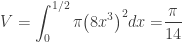
. on the interval [0, ½] is revolved around the x-axis to form a solid figure. Find the volume of this figure.
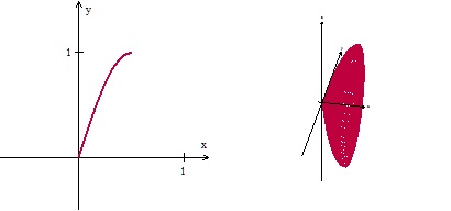

 on the interval [0, ½] is revolved around the x-axis to form a solid figure. Find the volume of this figure.
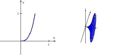


 .
. inside the integral sign so that each integrand looks like the formula for the area of a circle. What the students need to know is to subtract the volume hole from the outside volume. With that idea and the disk method they can do any volume by washers problem.
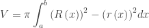 .
. is the area of and how it relates to this problem. See if the students can understand what the textbook is doing; what shape the book is using.. Discuss the Riemann sum approach. (MPAC 1 Reasoning with definitions and theorems, and MPAC 5 Notational fluency)
 and
and  is revolved around the x-axis. Find the volume of the resulting figure.


 and
and  from x = 1 to x = 5.
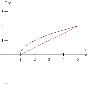
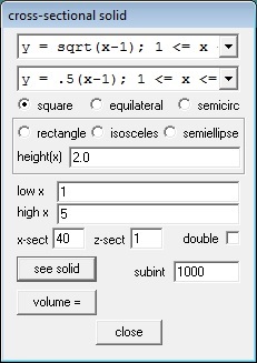
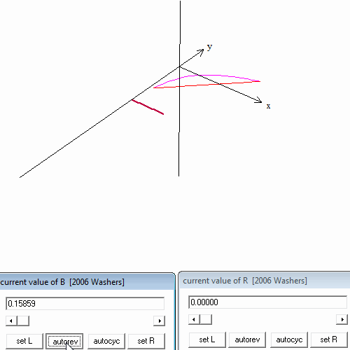
 Now let’s get fancy. Close the 3D window and return to the cross-section box shown above. Change the “high x” to 5@B (you may use any almost letter except x, y, or z). Then click “see solid.” Next, in the 3D Window click Anim > Individual > B. This will give you a slider. Slide the slider from 1 to 5 and you will see the solid grow and see the square cross-sections. (The video uses the “autocyc” button – use S to slow the animation, F to speed it up and Q to quit.)
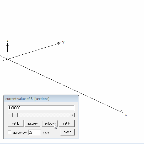


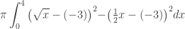
 , and the line
  between x = 0 and x = 4, revolved around
  .
. again revolved around