The Fundamental Theorem of Calculus

The Fundamental Theorem of Calculus or FTC, as its name suggests, is a very important idea. It is not sufficient to present the formula and show students how to use it. Show them where it comes from.

Here is an approach to demonstrate the FTC. I try to sneak up on the result by proposing a problem and then solving it. Here is the outline.

Suppose we have a differentiable function f that goes from \left( a,f\left( a \right) \right) to \left( b,f\left( b \right) \right). What is the net change in f over this interval? Easy it’s f\left( b \right)-f\left( a \right).  No problem, but way too easy for a calculus class. So let’s try a harder way!

Partition the interval [a, b] as you would for a Riemann sum, and calculate the change in f on each subinterval. The subintervals may be the same width or not. The change in y on the general subinterval [xi-1, xi] is f\left( {{x}_{i}} \right)-f\left( {{x}_{i-1}} \right).

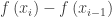
Approximate the net change over the whole interval by adding these \displaystyle \sum\limits_{i=1}^{n}{\left( f\left( {{x}_{i}} \right)-f\left( {{x}_{i-1}} \right) \right)} .
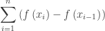
Is this a Riemann sum? No it is not! There is no \Delta x part. What to do?

The expression f\left( {{x}_{i}} \right)-f\left( {{x}_{i-1}} \right) looks familiar.
It is part of the equation for the Mean Value Theorem: \displaystyle {f}'\left( c \right)=\frac{f\left( b \right)-f\left( a \right)}{b-a} or {f}'\left( c \right)\left( b-a \right)=f\left( b \right)-f\left( a \right).
If we adapt this to the subinterval letting ci be the number guaranteed by the MVT on each subinterval  [xi-1, xi], then f\left( {{x}_{i}} \right)-f\left( {{x}_{i-1}} \right)={f}'\left( {{c}_{i}} \right)\left( {{x}_{i}}-{{x}_{i-1}} \right)

We can rewrite the sum in step 3 as \displaystyle \sum\limits_{i=1}^{n}{\left( f\left( {{x}_{i}} \right)-f\left( {{x}_{i-1}} \right) \right)}=\sum\limits_{n=1}^{n}{\left( {f}'\left( {{c}_{i}} \right)\left( {{x}_{i}}-{{x}_{i-1}} \right) \right)} .

  1. This is a Riemann sum and therefore, \displaystyle \underset{n\to \infty }{\mathop{\lim }}\,\sum\limits_{n=1}^{n}{\left( {f}'\left( {{c}_{i}} \right)\left( {{x}_{i}}-{{x}_{i-1}} \right) \right)}=\int_{a}^{b}{{f}'\left( c \right)dx} .
  2. So what is this equal to? We have already found what this limit is in step 1, so we now have:

\displaystyle \int_{a}^{b}{{f}'\left( x \right)dx}=f\left( b \right)-f\left( a \right).

This is called the FTC. And it is important.

The first thing it tells us is that the integral of a rate of change is the (net) amount of change. This will help us do a variety of problems.

The second thing it tells us is that, if we can find a function of which the integrand is the derivative (i.e. its antiderivative), then we can find the value of a definite integral by evaluating an antiderivative at the endpoints and subtracting. No more struggling with trying to find the limit of Riemann sums or graphing the function and hoping you can break it into regions with easy to find areas. All we need is an antiderivative and then one quick computation will do the trick from now on.

There is more to the FTC. This will be the subject of the next post.

The Definition of the Definite Integral

From the last post, it seems pretty obvious that as the number of rectangles in a Riemann sum increases or, what amounts to the same thing, the width of the sub-intervals decreases, the Riemann sum approaches the area of the region between a graph and the x-axis. The figures below show left-Riemann sums for the function f\left( x \right)=1+{{x}^{2}} on the interval [1, 4]. Hover and click on the figure below.

This slideshow requires JavaScript.

As the number of rectangles increases, they fill up more and more of the region. The sums increase, yet, their sum is always less than the area. They form an increasing sequence which is bounded above and therefore approaches its least upper bound (the area) as a limit.

Right-side rectangles work almost the same way. The sums form a decreasing sequence that is bounded below by the area and thus they approach the same limit.

All of the other Riemann sums must be between these two (at least for this example) and thus all approach the same limit.

This limit is called the definite integral for f on the interval [a, b], denoted by the new symbol below.

\displaystyle \underset{n\to \infty }{\mathop{\lim }}\,\sum\limits_{i=1}^{n}{f\left( x_{i}^{*} \right)\left( {{x}_{i}}-{{x}_{i-1}} \right)}=\underset{\Delta x\to 0}{\mathop{\lim }}\,\sum\limits_{i=1}^{n}{f\left( x_{i}^{*} \right)\Delta x=\int_{a}^{b}{f\left( x \right)dx}}

The notation has the advantage of being simpler to write than all the limit stuff and it shows us the interval which the limits do not. (For now consider the dx as a stand-in for \Delta x.)

The disadvantage of the notation is that, as we use it for real applications, the concept of Riemann sums often gets lost. The integrals become formulas and they get memorized but not understood.

Remember: behind every (any, all) definite integral is a Riemann sum.  As we look at applications, we should always look for the Riemann sum and how it is set up. This will tell us what the definite integral should be. We will not need to be too fussy about the subscripts and such; in fact, we will almost ignore them, but we will look carefully at the Riemann sum rectangles.

Riemann Sums

In our last post we discussed what are called Riemann sums. A sum of the form \displaystyle \sum\limits_{i=1}^{n}{f\left( x_{i}^{*} \right)\left( {{x}_{i}}-{{x}_{i-1}} \right)} or the form \sum\limits_{i=1}^{n}{f\left( x_{i}^{*} \right)\Delta x} (with the meanings from the previous post) is called a Riemann sum.

The three most common are these and depend on where the x_{i}^{*} is chosen.

  • Left-Riemann sum, L, uses the left side of each sub-interval, so x_{i}^{*}={{x}_{n-1}}.
  • Right-Riemann sum, R, uses the right side of each sub-interval, so x_{i}^{*}={{x}_{i}}.
  • Midpoint-Riemann sum, M, uses the midpoint of each interval, so x_{i}^{*}=\tfrac{1}{2}\left( {{x}_{i-1}}+{{x}_{i}} \right).

For the AP Exams students should know these and be able to compute them. The actual values are often given in a table, so the long computation of the function values is not necessary.

Another way of approximating the area between the graph and the x-axis is to use trapezoids formed by joining the points at the ends of each sub-interval. The areas can be figured individually and added or the value, T, can be found by averaging the left- and right-Riemann sums, T=\tfrac{1}{2}\left( L+R \right). This trapezoid approximation is usually closer to the true value than the other left- or right sums.

Whenever you are dealing with approximations, you should have some sense of how good they are. All of the approximations discussed will get closer to the true area if more values (more partition points) are used.

If the graph is increasing on the interval, then the left-sum is an underestimate of the actual value and the right-sum is an overestimate.  If the curve is decreasing, then the right-sums are underestimates and the left-sums are overestimates. (To see why, draw a sketch.)

If the graph is concave up the trapezoid approximation is an overestimate, and the midpoint is an underestimate. If the graph is concave down, then trapezoids give an underestimate and the midpoint an overestimate. (To see how this works, draw a sketch. For the midpoint draw the tangent line at the midpoint to the sides of the sub-interval; this trapezoid has the same area as the rectangle drawn at the midpoint of the interval. Why?)

If the graphs are not monotone on the interval or change concavity, then all bets are off.

For all of the Riemann sums, including those not mentioned above, as the number of partition points increase (n\to \infty ), or the width of the all the sub-interval decrease (\Delta x\to 0), the limit of a Riemann sum approaches the area between the graph and the x-axis. This will be the subject of the next post.


Corrected 11-28-2017


Working Towards Riemann Sums

In three previous posts (Nov 30, Dec 3 and Dec 5, 2012) we considered some examples leading up to integration and Riemann sums. Graphically all three can be seen as finding the area of the region between a graph and the x-axis over an interval.  The next thing to do is to abstract that process and see if we can do this in general for any continuous function.

Most all of the textbooks do this in the same way and that’s probably what you should now lead your students through. Start with the simple basic case of a function that is positive, monotone, and continuous on an interval [a, b]. You wish to approximate the area of the region between the graph and the x-axis with vertical sides at x = a and x = b. (The actual minimum conditions are only that the function be bounded and continuous at all but a finite number of points. But that can wait.)

Follow the steps in your textbook.

The things you should emphasize first with numbers and then eventually with symbols are these.

  1. The interval is divided into n sub-intervals each of equal length \Delta x=\frac{b-a}{n}.
  2. The x-coordinates of the endpoints are written in terms of a and \Delta x. This is called a partition of the interval. The x-coordinates are a={{x}_{0}}, {{x}_{1}}=a+(1)\Delta x, {{x}_{2}}=a+(2)\Delta x, {{x}_{3}}=a+(3)\Delta x up to {{x}_{n}}=a+(n)\Delta x=b.
  3. Decide on a scheme to evaluate the function a one point in each of the sub-intervals defined by the partition. This is usually done at the left or right endpoint, but in fact may be anywhere in the sub-interval. The notation for this “any point” is f\left( x_{i}^{*} \right), which may be a little complicated. If you decide on using the right end then for the ith sub-interval [{{x}_{i-1}},{{x}_{i}}] the value is f\left( {{x}_{i}} \right), for the left side the value is f\left( {{x}_{i-1}} \right). This is the vertical distance between the graph and the x-axis.
  4. Multiply this by the width of the sub-interval, this gives f\left( {{x}_{i}} \right)\Delta x. Do this for each sub-interval and add the results to get your approximation. For the right side approximation this looks like \sum\limits_{i=1}^{n}{f\left( {{x}_{i}} \right)\Delta x}.

Have your students compute this number for several functions with n in the 3 – 6 range. Your book will have plenty of examples. The idea is to learn and understand the procedure.

Some comments about each step above in case the kids ask. (Hope that they do.) Referring to the numbers above:

  1. The sub-intervals do not have to be the same length. When we get to taking limits of the sum above, the actual requirement is that whatever way we partition the interval the largest sub-interval (called the norm of the partition) approaches zero in length as n increases. For actually doing the computation, equal length sub-intervals are easiest.
  2. There will be a different \Delta x for each interval: \Delta {{x}_{i}}={{x}_{i}}-{{x}_{i-1}}.
  3. You may pick any point in a sub-interval, and you do not even have to pick the same way in each sub-interval. For computation, the right side is usually the easiest, with the left side not far behind. For the theory involved, picking the largest and/or smallest value in each sub-interval is used. This value may not be at an endpoint.
  4. Regardless of any of the above you will still multiply the function value by the width of the interval. The notation is more complicated. The sum is now written \sum\limits_{i=1}^{n}{f\left( x_{i}^{*} \right)\left( {{x}_{i}}-{{x}_{i-1}} \right)}

The important thing here is not the notation, but the process of partitioning the interval, calculating the function values multiplied by the width of the interval, and adding these products.

Under is a Long Way Down

The development of the ideas and concepts related to definite integrals almost always begins with finding the area of a region between a graph in the first quadrant and the x-axis between two vertical lines. Everyone, including me in the past, refers to this as “finding the area under the curve.”

Under is a long way down. And while everyone understands what this means, I suggest that a better phrasing is “finding the area between the curve and the x-axis.” Here is why:

  • That is what you are doing.
  • You will soon be finding the area between the curve and the x-axis where the curve is below the x-axis. This often leads to something you may be tempted to call “negative area” and of course there is no such thing as a negative area, regardless of what you may find in some textbooks.

As with so many integration problems, the results is often a formula that obscures what is really going on – the Riemann sum whose value the integral gives. The first such formula is that the area is given by \int_{a}^{b}{f\left( x \right)dx}. This is correct only if  f (x) > 0. There is a natural confusion for beginning students between the facts that if f (x) < 0 the integral comes out negative, but the area is positive.

For all the applications of integration always emphasize the Riemann sum – not just the final formula. In the area problem with f (x) > 0 the integrand is the vertical length of the rectangles that make up the sum and this is the upper function’s value minus the lower function’s value, with the lower being the x-axis, y = 0. Then when f (x) < 0 the upper minus the lower is 0 – f (x) and the area is given by \int_{a}^{b}{0-f\left( x \right)dx}=-\int_{a}^{b}{f\left( x \right)dx} which is positive as it should be. And students will immediately see that \int_{a}^{b}{f\left( x \right)dx} is not automatically the area.

To help students see this you could start (very first problem) by helping them to find the area of the region between f (x) > 0 and the line y = 1 so they have to deal with the lower curve. Then consider another problem using the x-axis.

There is a fair amount of ground to cover between the first area between the curve and the x-axis problems with f (x) > 0 and other area problems. Teaching students how to set up those first Riemann sums, what a Riemann sum is, the definition of the definite integral and even the Fundamental Theorem of Calculus may all come between the first problem and when this distinction becomes important. Starting with the right words, “area between the graph and the x-axis”, will help in the long run.