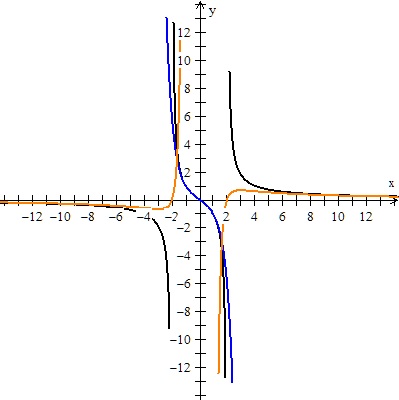
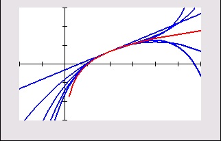
The polynomial function 


This is not a fluke!

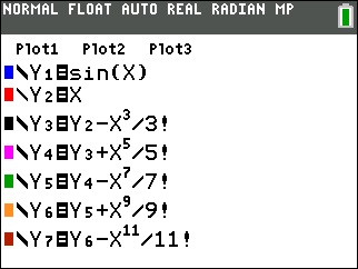
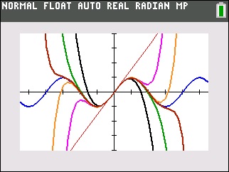
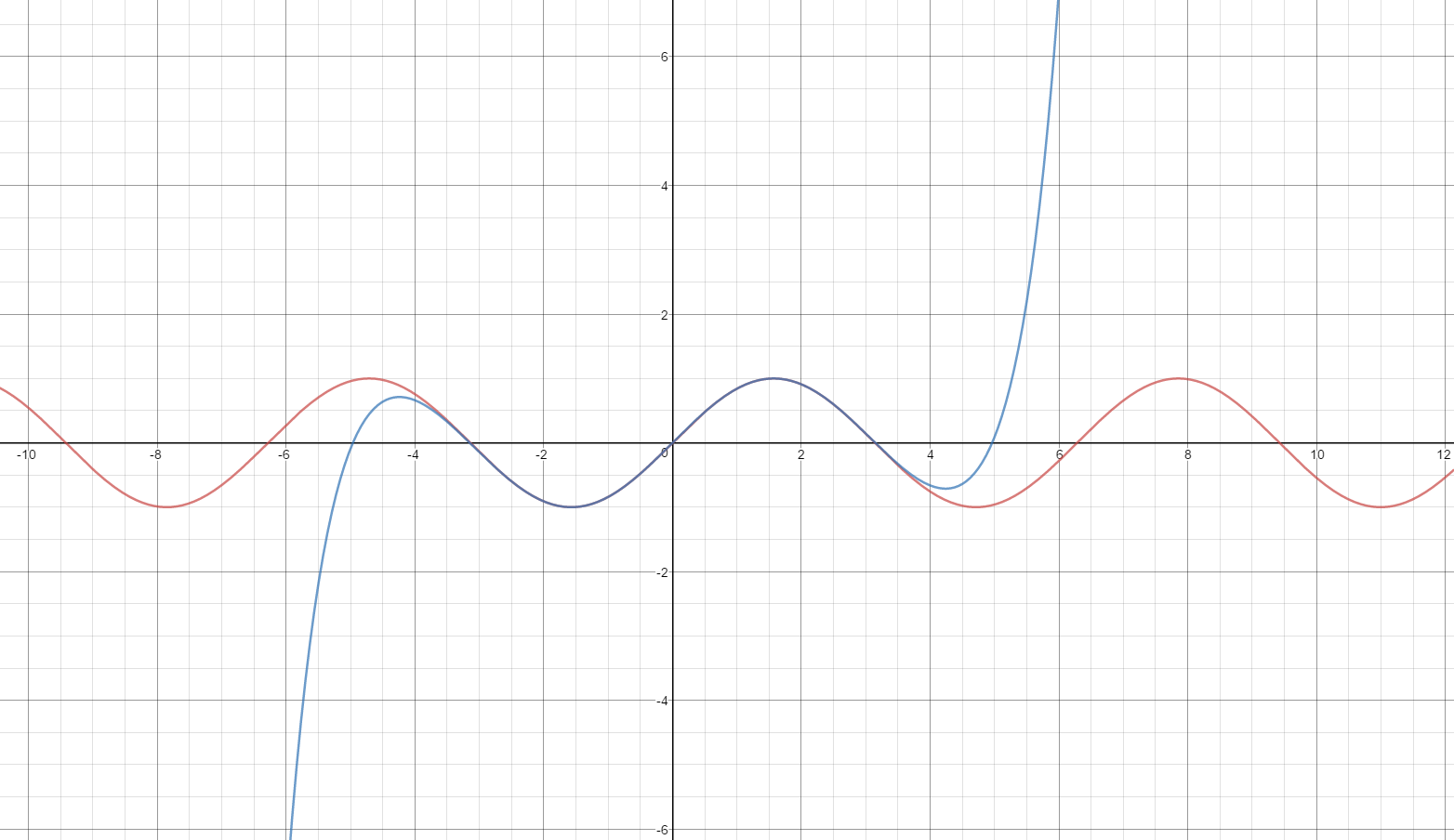
Now, approximating the value of a sine function is easier with a calculator. But sines are not the only functions in Math World.
In the Unit 10 you will learn how to write special polynomial functions, called Taylor and Maclaurin polynomials, to approximate any differentiable function you want to as many decimal places as you need. You already know a lot about polynomials. They are easy to understand, evaluate, and graph. The concept of using a polynomial to approximate much more complicated functions is very powerful.
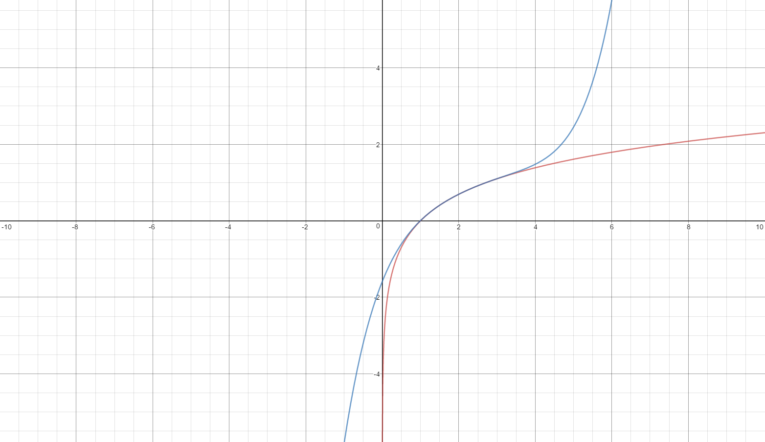
You’ve already got a start on this! Recall that the local linear approximation of a function near x = a is 
To fully understand these polynomials, there is a fair amount of preliminary stuff you need to understand. First you study sequences – functions whose domains are whole numbers. Next comes infinite series. A series is written by adding the terms of a sequence. (Sequences and series may have a finite or infinite number of terms. There is not much to say about finite series; infinite sequences and infinite series are where the action is.) oThe terms 0f some sequences and series are numbers. Other series have powers of an independent variable; these are called power series.
Some power series approximate (converge to) the related function everywhere (i. e. for all Real numbers). Others provide a good approximation only on an interval of finite length. The intervals where the approximation is good is called the interval of convergence. Convergence tests – theorems really – help you determine if a series converges. These in tern help you find the interval of convergence. More on this in my next post.
Depending on your textbook and your teacher, you may study these topics in this order: sequences, convergence test, series, Taylor and Maclaurin polynimials for approximations, and power series. Others may change the order. The path may be different, but the destination will be the same.
Course and Exam Description Unit 10, Sections 10.1, 10.2, 10.11, 10.13, 10.14, 10.15. This is a BC only topic.
 , sin(x), cos(x), and ex.
 , sin(x), cos(x), and ex
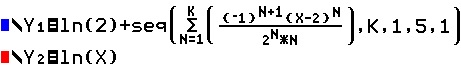
 , instead of cranking out a bunch of derivatives, we can say this looks a lot like the formula for the sum of a geometric series,
 . Taking a = 3x and r = 2x, the series is
 .
. , the interval of convergence for this series is
  or
or  and we don’t even have to check the endpoints.
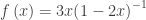 and then expand the binomial using the binomial theorem. Or we could use the technique of long division of polynomials to divide 3x by (1 – 2x) – leaving the divisor as written here.
 . Begin by dividing each term by –4. This gives
 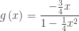 . Then treating this as a geometric series
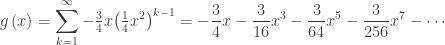
 , or –2 < x < 2
 and then wrote:
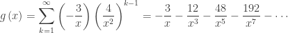
 , or
, or  , or the union of
  and
and  , Whoa, that’s different and not even an interval.