Good Question 6: 2000 AB 4

Posted on August 25, 2015 by Lin McMullin

Another of my favorite questions from past AP exams is from 2000 question AB 4. If memory serves it is the first of what became known as an “In-out” question. An “In-out” question has two rates that are working in opposite ways, one filling a tank and the other draining it.

In subsequent years we saw a question with people entering and leaving an amusement park (2002 AB2/BC2), sand moving on and off a beach (2005 AB 2), another tank (2007 AB2), an oil leak being cleaned up (2008 AB 3), snow falling and being plowed (2010 AB 1), gravel being processed (2013 AB1/BC1), and most recently water again flowing in and out of a pipe (2015 AB1/BC1). The in-between years saw rates in one direction only but featured many of the same concepts.

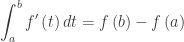
The questions give rates and ask about how the quantity is changing. As such, they may be approached as differential equation initial value problems, but there is an easier way. This easier way is that a differential equation that gives the derivative as a function of a single variable, t, with an initial point $\left( {{t}_{0}},y\left( {{t}_{0}} \right) \right)$ always has a solution of the form

$y\left( t \right)=y\left( {{t}_{0}} \right)+\int_{{{t}_{0}}}^{t}{{y}'\left( x \right)dx}$ .

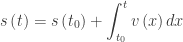
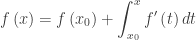
This is sometimes called the “accumulation equation.” The integral of a rate of change ${y}'\left( t \right)$ gives the net amount of change over the interval of integration $[{{t}_{0}},t]$ . When this is added to the initial amount the result is an expression that gives the amount at any time t.

In a motion context, this same idea is that the position at any time t, is the initial position plus the displacement:

$\displaystyle s\left( t \right)=s\left( {{t}_{0}} \right)+\int_{{{t}_{0}}}^{t}{v\left( x \right)dx}$ where $v\left( t \right)={s}'\left( t \right)$

The scoring standard gave both forms of the solution. The ease of the accumulation form over the differential equation solution was evident and subsequent standards only showed this one.

2000 AB 4

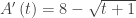
The question concerned a tank that initially contained 30 gallons of water. We are told that water is being pumped into the tank at a constant rate of 8 gallons per minute and the water is leaking out at the rate of $\sqrt{t+1}$ gallons per minute.

Part a asked students to compute the amount of water that leaked out in the first three minutes. There were two solutions given. The second solves the problem as an initial value differential equation:

Let L(t) be the amount that leaks out in t minutes then

$\displaystyle \frac{dL}{dt}=\sqrt{t+1}$

$L\left( t \right)=\frac{2}{3}{{\left( t+1 \right)}^{3/2}}+C$

$L\left( 0 \right)=\frac{2}{3}{{\left( 0+1 \right)}^{3/2}}+C=0$ since nothing has leaked out yet, so C = -2/3

$L\left( t \right)=\frac{2}{3}{{\left( t+1 \right)}^{3/2}}-\frac{2}{3}$

$L\left( 3 \right)=\frac{14}{3}$

The first method, using the accumulation idea takes a single line:

$\displaystyle L\left( 3 \right)=\int_{0}^{3}{\sqrt{t+1}dt}=\left. \frac{2}{3}{{\left( t+1 \right)}^{3/2}} \right|_{0}^{3}=\frac{2}{3}{{\left( 4 \right)}^{3/2}}-\frac{2}{3}{{\left( 1 \right)}^{3/2}}=\frac{14}{3}$

I think you’ll agree this is easier and more direct.

Part b asked how much water was in the tank at t = 3 minutes. We have 30 gallons to start plus 8(3) gallons pumped in and 14/3 gallons leaked out gives 30 + 24 – 14/3 = 148/3 gallons.

This part, worth only 1 point, was a sort of hint for the next part of the question.

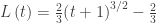
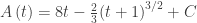
Part c asked students to write an expression for the total number of gallons in the tank at time t.

Following part b the accumulation approach gives either

$\displaystyle A\left( t \right)=30+8t-\int_{0}^{t}{\sqrt{x+1}dx}$ or

$\displaystyle A\left( t \right)=30+\int_{0}^{t}{\left( 8-\sqrt{x+1} \right)dx}$ .

The first form is not a simplification of the second, but rather the second form is treating the difference of the two rates, in minus out, as the rate to be integrated.

The differential equation approach is much longer and looks like this:

$\displaystyle \frac{dA}{dt}=8-\sqrt{t+1}$

$A\left( t \right)=8t-\frac{2}{3}{{\left( t+1 \right)}^{3/2}}+C$

$A\left( 0 \right)=30=8(0)-\frac{2}{3}{{\left( 0+1 \right)}^{3/2}}+C$ , so $C=\frac{92}{3}$

$A\left( t \right)=8t-\frac{2}{3}{{\left( t+1 \right)}^{3/2}}+\frac{92}{3}$

Again, this is much longer. In recent years when asking student to write an expression such as this, the directions included a phrase such as “write an equation involving one or more integrals that gives ….” This pretty much leads students away from the longer differential equation initial value problem approach.

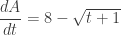
Part d required students to find the time when in the interval $0\le t\le 120$ minutes the amount of water in the tank was a maximum and to justify their answer. The usual method is to find the derivative of the amount, A(t), set it equal to zero, and then solve for the time.

${A}'\left( t \right)=8-\sqrt{t+1}$

Notice that this is the same regardless of which of the three forms of the expression for A(t) you start with. Thus, an excellent example of the Fundamental Theorem of Calculus used to find the derivative of a function defined by an integral. Or you could just start here without reference to the forms above: the overall rate in the rate in minus the rate out.

${A}'\left( t \right)=0$ when t = 63

This is a maximum by the First Derivative Test since for 0 < t < 63 the derivative of A is positive and for 63 < t <120 the derivative of A is negative.

There is an additional idea on this part of the question in the Teaching Suggestions below.

I like this question because it is a nice real (as real as you can hope for on an exam) situation and for the way the students are led through the problem. I also like the way it can be used to compare the two methods of solution. Then the way they both lead to the same derivative in part d is nice as well. I use this one a lot when working with teachers in workshops and summer institutes for these very reasons.

Teaching Suggestions

Certainly, have your students work through the problem using both methods. They need to learn how to solve an initial value problem (IVP) and this is good practice. Additionally, it may help them see how and when to use one method or the other.
Be sure the students understand why the three forms of A(t) in part c give the same derivative in part d. This makes an important connection with the Fundamental theorem of Calculus.
Like many good AP questions part d can be answered without reference to the other parts. The question starts with more water being pumped in than leaking out. This will continue until the rate at which the water leaks out overtakes the rate at which it is being pumped in. At that instant the rate “in” equals the rate “out” so you could start with $8=\sqrt{t+1}$ . After finding that t = 63, the answer may be justified by stating that before this time more water is being pumped in than is leaking out and after this time the rate at which water leaks out is greater than the rate at which it is pumped in, so the maximum must occur at t = 63.
And as always, consider the graph of the rates.

I used this question as the basis of a lesson in the current AP Calculus Curriculum Module entitled Integration, Problem Solving and Multiple Representations © 2013 by the College Board. The lesson gives a Socratic type approach to this question with a number of questions for each part intended to help the teacher not only work through this problem but to bring out related ideas and concepts that are not in the basic question. The module is currently available at AP sponsored workshops and AP Summer Institutes. Eventually, it will be posted at AP Central on the AB and BC Calculus Home Pages.

The Rate/Accumulation Question

Posted on March 1, 2013 by Lin McMullin

AP Type Questions 1

These questions are often in context with a lot of words describing a situation in which some things are changing. There are usually two rates given acting in opposite ways. Students are asked about the change that the rates produce over some time interval either separately or together.

The rates are often fairly complicated functions. If they are on the calculator allowed section, students should store them in the equation editor of their calculator and use their calculator to do any integration or differentiation that may be necessary.

The integral of a rate of change is the net amount of change

$\displaystyle \int_{a}^{b}{{f}'\left( t \right)dt}=f\left( b \right)-f\left( a \right)$

over the time interval [a, b]. If the question asked for an amount, look around for a rate to integrate.

The final accumulated amount is the initial amount plus the accumulated change:

$\displaystyle f\left( x \right)=f\left( {{x}_{0}} \right)+\int_{{{x}_{0}}}^{x}{{f}'\left( t \right)}\,dt$ ,

where ${{x}_{0}}$ is the initial time, and $f\left( {{x}_{0}} \right)$ is the initial amount. Since this is one of the main interpretations of the definite integral the concept may come up in a variety of situations.

What students should be able to do:

Be ready to read and apply; often these problems contain a lot of writing which needs to be carefully read.
Recognize that rate = derivative.
Recognize a rate from the units given without the words “rate” or “derivative.”
Find the change in an amount by integrating the rate. The integral of a rate of change gives the amount of change (FTC):

$\displaystyle \int_{a}^{b}{{f}'\left( t \right)dt}=f\left( b \right)-f\left( a \right)$ .

Find the final amount by adding the initial amount to the amount found by integrating the rate. If $x={{x}_{0}}$ is the initial time, and $f\left( {{x}_{0}} \right)$ is the initial amount, then final accumulated amount is

$\displaystyle f\left( x \right)=f\left( {{x}_{0}} \right)+\int_{{{x}_{0}}}^{x}{{f}'\left( t \right)}\,dt$ ,

Understand the question. It is often not necessary to as much computation as it seems at first.
Use FTC to differentiate a function defined by an integral.
Explain the meaning of a derivative or its value in terms of the context of the problem.
Explain the meaning of a definite integral or its value in terms of the context of the problem. The explanation should contain (1) what it represents, (2) its units, and (3) how the limits of integration apply in context.
Store functions in their calculator recall them to do computations on their calculator.
If the rates are given in a table, be ready to approximate an integral using a Riemann sum or by trapezoids.
Do a max/min or increasing/decreasing analysis.

Shorter questions on this concept appear in the multiple-choice sections. As always, look over as many questions of this kind from past exams as you can find.

For some previous posts on this subject see January 21, 23, 2013

Painting a Point

Posted on February 4, 2013 by Lin McMullin

Accumulation 7: An application (of paint)

Suppose you started with a point, the origin to be specific, and painted it. You put on layers and layers of paint until your point grows to a sphere with radius r. Let’s stop and admire your work part way through the job; at this point the radius is ${{x}_{i}}$ and $0\le {{x}_{i}}\le r$ .

How much paint will you need for the next layer?

Easy: you need an amount equal to the surface area of the sphere, $4\pi {{x}_{i}}^{2}$ , times the thickness of the paint. As everyone knows paint is thin, specifically $\Delta x$ thin. So we add an amount of paint to the sphere equal to $4\pi {{x}^{2}}\left( \Delta x \right)$ .

The volume of the final sphere must be the same as the total amount of paint. The total amount of paint must be the (Riemann) sum of all the layers or $\displaystyle \sum\limits_{i=1}^{n}{4\pi {{x}_{i}}^{2}\left( \Delta x \right)}$ . As usual $\Delta x$ is very thin, tending to zero as a matter of fact, so the amount of paint must be

$\displaystyle \underset{\Delta x\to 0}{\mathop{\lim }}\,\sum\limits_{i=1}^{n}{4\pi {{x}_{i}}^{2}\left( \Delta x \right)=\int_{0}^{r}{4\pi {{x}^{2}}}dx=\left. \tfrac{4}{3}\pi {{x}^{3}} \right|_{0}^{r}=\tfrac{4}{3}\pi {{r}^{3}}}$ .

A standard related rate problem is to show that the rate of change of the volume of a sphere is proportional to its surface area – the constant of proportionality is dr/dt. So it should not be a surprise that the integral of this rate of change of the surface area is the volume. The integral of a rate of change is the amount of change.

Interestingly this approach works other places as long as you properly define “radius:”

A circle centered at the origin with radius x and perimeter of $2\pi x$ , gains area at a rate equal to its perimeter times the “thickness of the edge” $\Delta x$ : $\displaystyle A=\underset{n\to \infty }{\mathop{\lim }}\,\sum\limits_{k=1}^{n}{2\pi x\Delta x}=\int_{0}^{r}{2\pi x\,dx=\pi {{r}^{2}}}$

A square centered at the origin with “radius” x with sides whose length are s =2 x, gains area at a rate equal to its perimeter (8x) times the “thickness of the edge” $\Delta x$ : $\displaystyle A=\underset{n\to \infty }{\mathop{\text{lim}}}\,\sum\limits_{k=1}^{n}{8x\Delta x=\int_{0}^{x}{8x\,dx}}=4{{x}^{2}}={{(2x)}^{2}}={{s}^{2}}$

A cube centered at the origin with “radius” x and edges of length 2x, gains volume at a rate equal to its surface area, $6(4{{x}^{2}})$ , times the “thickness of the face” $\Delta x$ – think paint again: $V=\underset{n\to \infty }{\mathop{\text{lim}}}\,\sum\limits_{k=1}^{n}{\text{6(4}{{\text{x}}^{2}})\Delta x}=\int_{0}^{x}{24{{x}^{2}}dx}=8{{x}^{3}}={{(2x)}^{3}}={{s}^{3}}$

Stamp Out Slope-intercept Form!

Posted on January 30, 2013 by Lin McMullin

Accumulation 5: Lines

If you have a function y(x), that has a constant derivative, m, and contains the point $\left( {{x}_{0}},{{y}_{0}} \right)$ then, using the accumulation idea I’ve been discussing in my last few posts, its equation is

$\displaystyle y={{y}_{0}}+\int_{{{x}_{0}}}^{x}{m\,dt}$

$\displaystyle y={{y}_{0}}+\left. mt \right|_{{{x}_{0}}}^{x}$

$\displaystyle y={{y}_{0}}+m\left( x-{{x}_{0}} \right)$

This is why I need your help!

I want to ban all use of the slope-intercept form, y = mx + b, as a method for writing the equation of a line!

The reason is that using the point-slope form to write the equation of a line is much more efficient and quicker. Given a point $\left( {{x}_{0}},{{y}_{0}} \right)$ and the slope, m, it is much easier to substitute into $y={{y}_{0}}+m\left( x-{{x}_{0}} \right)$ at which point you are done; you have an equation of the line.

Algebra 1 books, for some reason that is beyond my understanding, insist using the slope-intercept method. You begin by substituting the slope into $y=mx+b$ and then substituting the coordinates of the point into the resulting equation, and then solving for b, and then writing the equation all over again, this time with only m and b substituted. It’s an algorithm. Okay, it’s short and easy enough to do, but why bother when you can have the equation in one step?

Where else do you learn the special case (slope-intercept) before, long before, you learn the general case (point-slope)?

Even if you are given the slope and y-intercept, you can write $y=b+m\left( x-0 \right)$ .

If for some reason you need the equation in slope-intercept form, you can always “simplify” the point-slope form.

But don’t you need slope-intercept to graph? No, you don’t. Given the point-slope form you can easily identify a point on the line, $\left( {{x}_{0}},{{y}_{0}} \right)$ , start there and use the slope to move to another point. That is the same thing you do using the slope-intercept form except you don’t have to keep reminding your kids that the y-intercept, b, is really the point (0, b) and that’s where you start. Then there is the little problem of what do you do if zero is not in the domain of your problem.

Help me. Please talk to your colleagues who teach pre-algebra, Algebra 1, Geometry, Algebra 2 and pre-calculus. Help them get the kids off on the right foot.

Whenever I mention this to AP Calculus teachers they all agree with me. Whenever you grade the AP Calculus exams you see kids starting with y = mx + b and making algebra mistakes finding b.

Graphing with Accumulation 2

Posted on January 28, 2013 by Lin McMullin

Accumulation 4: Graphing Ideas in Accumulation – Concavity

In the last post we saw how thinking about Riemann sum rectangles, RΣR, moving across the graph of the derivative made it easy to see when the function whose derivative was given increased and decreased and had its local extreme values. Today we will consider concavity.

Suppose a derivative is constant, its graph a horizontal line. In this case each successive RΣR is exactly the same size and adds exactly the same amount to the accumulated function. The function’s graph increases (or decreases) by exactly the same amount – it is linear.

For derivatives that are not constant, the change in the resulting function is not constant and the function’s graph bends up or down. This bending of the function is referred to as its concavity. If it bends up, the function increases faster and its graph is concave up; if it bends down, it is increasing slower (or decreasing faster) and concave down.

The graph above shows pairs of RΣR in different intervals as they move along the graph of a derivative. Consider the dark blue rectangle to be the previous position of the red rectangle.

As the RΣR moves from a to b each red rectangle is larger than the dark blue one. Each move adds more to the accumulated sum than the previous one. The graph of the function increases more with each move – it is concave up.

As the RΣR moves from b to d (there are two pairs drawn) each red RΣR has a smaller value than the previous one. (Remember when they are below the x-axis the longer (red) RΣR has a smaller value.) In the interval [b, d] less is added to the accumulated sum (or more is subtracted) with each move to the right. Therefore, the graph of the function bends down – the function is concave down.

In the last section, from d to f the red rectangle now has a larger value than the dark blue one. (Again, remember that when the function has negative values, the shorter rectangle, has the larger value.) The graph of the function again bends up – is concave up.

Putting these ideas together with those in the last post we can see how the moving RΣR idea can distinguish the four shapes of the graph of the accumulating function:

On [a, b] the function’s graph is increasing and concave up; the RΣR are positive and getting more positive (longer).

On [b, c] the function’s graph is increasing and concave down; the RΣR are positive and getting less positive (shorter).

On [c, d] the function’s graph is decreasing and concave down; the RΣR are negative and getting more negative (longer).

On [d, e] the function’s graph is decreasing and concave up; the RΣR are negative and getting less negative (shorter).

At the extreme values of the derivative, the concavity of the function changes from up to down or down to up. These are called points of inflection.

Questions in which students are asked about the properties of a function given the graph, but not the equation, of the derivative are very common. Many students (including me) find this approach easier and more intuitive than working strictly with derivative ideas.

Graphing with Accumulation 1

Posted on January 25, 2013 by Lin McMullin

Accumulation 3: Graphing Ideas in Accumulation – Increasing and decreasing

Previously, we discussed how to determine features of the graph of a function from the graph of its derivative. This required knowing (memorizing) and understanding facts about the derivative (such as the derivative is negative) and how they related to the graph of the function (the function was decreasing). There is another method that I prefer. I find that using the accumulation idea it is easy to “see” what the function is doing.

Consider the graph of the derivative of a function and picture one Riemann sum rectangle (RΣR) as it moves from left to right across the graph. If the derivative is positive the RΣR will have a positive value and if the derivative is negative the RΣR will have a negative value. Each RΣR adds to or subtracts from the accumulated value that is represented by the function.

In the drawing above we see the graph of a derivative with a RΣR drawn at three places. At a the function has some initial value which may be 0. As the RΣR moves from a to c the RΣR have a positive value and each one adds a little to the function’s value. The function accumulates value and increases.

As the RΣR moves from c to e the value of the RΣR is negative and thus subtracts from the accumulating value, so the function decreases.

In the interval e to g the RΣR once again is positive so the accumulating value increases.

At c the RΣR changes from a positive value to a negative value, the function changes from increasing to decreasing: a local maximum. A similar thing happens at e, the RΣR changes from negative to positive, the function changes from decreasing to increasing: a local minimum.

To see and determine where the function is increasing and decreasing from the graph of its derivative, just picture the RΣR sliding left to right across the graph, each one adding to or subtracting from the accumulated value which is the function.

Often there are AP Calculus exam questions that show a derivative made up of segments or parts of circles. It is possible to find the area of the regions between the derivative and the x-axis. Starting on the extreme left side add or subtract the areas of the region to find the exact function values. If the left side value is not given (that is, some other place is the initial condition), treat the left-end value as a variable and add or subtract until you get to the initial value, and solve for the variable.

Next: Accumulation and concavity

AP Accumulation Questions

Posted on January 23, 2013 by Lin McMullin

Accumulation 2: AP Exam Rate/Accumulation Questions

I assume that a number of my readers are AP Calculus teachers. In following up my last post on accumulation, today I’m going to discuss a very common type of AP Calculus exam question, the rate question which is loaded with accumulation ideas. The three posts following this one will show how accumulation can help with graphing problems.

If you do not have them, these two links will take you to them. Click on the question number for links to the question and scoring standard.

2000 AB 4: In this questions water was being pumped into a tank at the constant rate of 8 gallons per minute and leaking out at the rate of $\sqrt{t+1}$ gallons per minute. At time t = 0 we are told there are 30 gallons of water in the tank. (Many AP exams problems have two rates acting at the same time, one increasing the amount and the other decreasing it.)

The first part of the question asked for the amount of water that leaked out of the tank in the first 3 minutes. This is like the situation discussed in the last post: If you need an amount, look around for a rate to integrate. The answer is $\displaystyle\int_{0}^{3}{\sqrt{t+1}dt}=\tfrac{14}{3}\text{ gallons}\text{.}$

The next part asked for the amount of water in the tank after t minutes. So, we start with 30 gallons and add the amount put in which is 8 gallons per minute for 3 minutes of 24 gallons. Of course, we could also get this by integrating $\displaystyle \int_{0}^{3}{8dt}=24$ . Then we subtract the amount that leaked out from the first part. The amount is 30 + 24 – 14/3 gallons. This was to help students with the next part.

The third part asked for an expression for A(t), the amount of water at any time t. So following on the second part we have either $\displaystyle A\left( t \right)=30+8t-\int_{0}^{x}{\sqrt{t+1}dt}$ or $\displaystyle A\left( t \right)=30+\int_{0}^{x}{8-\sqrt{t+1}\,dt}$ . Either form, especially the latter, is the form of an accumulation function: the initial amount plus the integral of the rate of change. It was not required to actually do the integration, but if someone did then $\displaystyle A\left( t \right)=8t-\tfrac{2}{3}{{\left( t+1 \right)}^{3/2}}+\tfrac{92}{3}$

The last part asked when the maximum amount of water was in the tank. As in any extreme value problem you can find this by differentiating any of the expressions for the amount found in the third part: ${A}'\left( t \right)=8-\sqrt{t+1}$ by the FTC. (This could also be found by simply subtracting the two rates.) This will change from positive to negative when t = 63; this is when the maximum amount of water is in the tank. Notice that this is when the amount leaking out becomes greater than the amount being pumped into the tank; the total change becomes negative.

2009 AB 3: This question had a different twist or two on the accumulation idea. This proved rather difficult for the majority of the students (The mean score was 1.92 out of a possible 9 points.) The problem said that the Mighty Cable Company sold their cable for $120 per meter. The cost of producing the cable was given as $6\sqrt{x}$ dollars per meter. (Notice that these are rates as evidenced by their units $/m; the word “rate” was not used. It is important that students recognize when something is a rate.) The stem also defined profit as the difference between the amount of money received for the cable and the cost of producing the cable.

The first part of the question asked for the profit on 25 meters of cable. The amount the company receives is 25 meters times $120 dollars per meter (an amount so we could integrate the rate here, but that’s overkill). The amount the 25 meters costs to produce is (remember if you need an amount, integrate the rate): $\displaystyle \int_{0}^{25}{6\sqrt{x}\,dx}$ , so the $\displaystyle \text{Profit }=120\cdot 25-\int_{0}^{25}{6\sqrt{x}\,dx}=\$2,500$

The third part built on the first part by asking for the profit earned for a cable k meters long: $\displaystyle \text{Profit =}120k-\int_{0}^{k}{6\sqrt{x}\,dx}$ or $\displaystyle P(x)=\int_{0}^{k}{120-6\sqrt{x}\,dx}$ . There is your accumulation function. The initial value is $0.

The second part was the most interesting. In it students were asked to explain the meaning of $\displaystyle \int_{25}^{30}{6\sqrt{x}\,dx}$ in the context of the problem. One way to see what this represents is to think about the FTC. The integral of the rate in dollars per meter is the cost per meter. If we call the cost C, then $\displaystyle \int_{25}^{30}{6\sqrt{x}\,dx}=C\left( 30 \right)-C\left( 25 \right)$ . 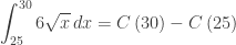Now students did not need to do a computation here; they just have to read what the symbols mean. $C\left( 30 \right)-C\left( 25 \right)$ is the difference between the cost of manufacturing a 25-meter cable and a 30-meter table. When you integrate a rate, you get the net amount.

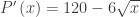
As in the previous question the fourth part asked for the maximum profit. This was found by differentiating the profit expression from the third part by the FTC, ${P}'\left( x \right)=120-6\sqrt{x}$ and finding when the derivative changed from positive to negative, at x = 400 meters and substituting this into the profit equation.

Teaching Calculus

The pleasure lies not in discovering the truth, but in searching for it.

Tag Archives: accumulation

Good Question 6: 2000 AB 4

The Rate/Accumulation Question

Stamp Out Slope-intercept Form!

Graphing with Accumulation 2

Graphing with Accumulation 1

AP Accumulation Questions

Share this:

Share this:

Share this:

Share this:

Share this:

Share this:

Share this: