Accumulation 3: Graphing Ideas in Accumulation – Increasing and decreasing

Previously, we discussed how to determine features of the graph of a function from the graph of its derivative. This required knowing (memorizing) and understanding facts about the derivative (such as the derivative is negative) and how they related to the graph of the function (the function was decreasing). There is another method that I prefer. I find that using the accumulation idea it is easy to “see” what the function is doing.

Consider the graph of the derivative of a function and picture one Riemann sum rectangle (RΣR) as it moves from left to right across the graph. If the derivative is positive the RΣR will have a positive value and if the derivative is negative the RΣR will have a negative value. Each RΣR adds to or subtracts from the accumulated value that is represented by the function.

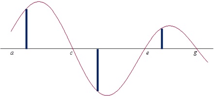
In the drawing above we see the graph of a derivative with a RΣR drawn at three places. At a the function has some initial value which may be 0. As the RΣR moves from a to c the RΣR have a positive value and each one adds a little to the function’s value. The function accumulates value and increases.

As the RΣR moves from c to e the value of the RΣR is negative and thus subtracts from the accumulating value, so the function decreases.

In the interval e to g the RΣR once again is positive so the accumulating value increases.

At c the RΣR changes from a positive value to a negative value, the function changes from increasing to decreasing: a local maximum. A similar thing happens at e, the RΣR changes from negative to positive, the function changes from decreasing to increasing: a local minimum.

To see and determine where the function is increasing and decreasing from the graph of its derivative, just picture the RΣR sliding left to right across the graph, each one adding to or subtracting from the accumulated value which is the function.

Often there are AP Calculus exam questions that show a derivative made up of segments or parts of circles. It is possible to find the area of the regions between the derivative and the x-axis. Starting on the extreme left side add or subtract the areas of the region to find the exact function values. If the left side value is not given (that is, some other place is the initial condition), treat the left-end value as a variable and add or subtract until you get to the initial value, and solve for the variable.

Next: Accumulation and concavity