Right Answer – Wrong Question

About this time every year the AP Calculus Community discussion turns to the sentence, “A function is continuous on its domain.” Functions such as f\left( x \right)=\frac{1}{x} cause confusion – is it continuous or not?  The confusion comes, I think, from the way we introduce continuity to new calculus students.

We say – and I did say this myself just last week – that the graph of a continuous function can be drawn without taking your pencil off the paper. That idea helps students get a start on understanding what continuity means, but it is not quite correct.

The definition of continuity requires that for a function to be continuous at a point, the limit at that point equals the value there (and that both the limit and value be finite). The only way a function can have a value at a point is if the point is in the domain. So, the definition of continuity can be applied only at points in the domain. If the domain of the function is not all Real numbers, then the function cannot be continuous “everywhere;” rather it can only be continuous on its domain. (And, of course, there are many examples of functions that are not continuous at all points in their domains.)

So what do you say about a function like f\left( x \right)=\frac{1}{x}?

Its domain is all Real numbers x\ne 0. The function is continuous at all the points in its domain and so it is continuous on its domain.

But that statement does not tell the whole story. We asked the wrong question. We should ask where the function is not continuous. If we ask where this function is not continuous, the answer is that the function is not continuous at x = 0. Asking where a function is not continuous requires that we consider the entire number line, all Real numbers. The answer often provides better information.

So then, obviously a function is not continuous at any and all the points not in its domain (plus perhaps some other points in its domain). Accepting that a function is continuous on its domain, even if correct, does give us as much information as asking where a function is not continuous.

Ask the right question!

Continuity 2

The definition of continuity of a function used in most first-year calculus textbooks reads something like this:

A function f is continuous at x = a if, and only if,

(1) f(a) exists (the value is a finite number),

(2) \underset{x\to a}{\mathop{\lim }}\,f\left( x \right) exists (the limit is a finite number), and

(3) \underset{x\to a}{\mathop{\lim }}\,f\left( x \right)=f\left( a \right) (the limit equals the value).

A function is continuous on an interval if, and only if, it is continuous at all values of the interval. For the endpoints of closed intervals, the limits are adjusted to one-sided limits with x approaching a from inside the interval.

As I’ve written before, limits logically come before continuity since limits are used in the definition of continuity. But as a practical and historical matter continuity comes first. Continuity, or rather lack of continuity, gives us the examples that motivate the need for the concept of limit.

Karl Weierstrass (1815 – 1897) gave the modern definition of continuity: Given a function f and an element a of the domain I,   f is said to be continuous at the point a if for any number \varepsilon >0, however small, there exists a number \delta >0 such that for all x in the domain of f\left| x-a \right|<\delta  implies \left| f\left( x \right)-f\left( a \right) \right|<\varepsilon .

This looks very much like the definition of limit. In the delta-epsilon definition of limit the last inequality above is \left| f\left( x \right)-L \right|<\varepsilon  where L is the limit. Replacing the value with the limit allows a somewhat simpler wording of the definition of continuity than that given at the beginning, but adds the delta-epsilon complication. Weierstrass’ definition eliminates the need for saying the value and the limit are finite since that is assumed by writing f (a).

Some textbooks use the phrase “a function is continuous on its domain.” This seems somewhat limiting (no pun intended) in that a function such as \displaystyle f\left( x \right)=\tfrac{1}{x} is certainly continuous on its domain but not continuous on the entire number line. We are usually concerned about where a function is not continuous, so first we find where it is not continuous: at the points not in its domain plus possibly other points in its domain.

Recent AP calculus exams (2012 AB4c, 2011 AB 6a) gave students a piecewise defined function and asked if it is continuous at the point where the two pieces meet. The question directed students to “use the definition of continuity to explain your answer” and “show that f is continuous.”  To answer the question students were expected to state what the two one-sided limits are and what the value there is. Since all these numbers are finite and equal the requirements of the definition are met.

This kind of question could be considered a question about continuity or a question about applying a definition (or theorem) to a particular situation. Either way students should understand the hypotheses of a definition or theorem and know how to verify that they are met in a particular situation.

L’Hôpital Rules the Graph

In my last post on May 31, 2012 I showed a way of demonstrating why L’Hôpital’s Rule works. We looked at an example,

\displaystyle \underset{x\to \pi }{\mathop{\lim }}\,\frac{\tan \left( x \right)}{\sin \left( x \right)},

which met the requirement of the theorem called L’Hôpital’s Rule, namely the functions are differentiable and, since  tan(\pi ) = sin(\pi ) = 0 they intersect on the x-axis at \left( \pi ,0 \right). We looked at the graph and then zoomed-in at
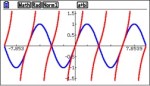
 \left( \pi ,0 \right).

L’Hôpital’s Rule tells us that with these conditions the limit is the same as the limit of the ratio of their slopes (or their derivatives, if you prefer). Can you see what that ratio is from Figure 2? Even though this is not a “square window” the ratio is obviously –1.

Here are four other limits. See if you can find them by the method suggested here. Namely zoom-in on the point where the functions intersect and see if you can find the limits without doing any computations. (Yes, I know you already know the first 3, but try this idea anyway. )

1. \displaystyle \underset{x\to 0}{\mathop{\lim }}\,\frac{\sin \left( x \right)}{x}

2. \displaystyle \underset{x\to 0}{\mathop{\lim }}\,\frac{1-\cos \left( x \right)}{x}

3. \displaystyle \underset{x\to 0}{\mathop{\lim }}\,\frac{\cos \left( \tfrac{\pi }{2}+x \right)}{x} also known as \displaystyle \underset{x\to 0}{\mathop{\lim }}\,\frac{\cos \left( \tfrac{\pi }{2}+x \right)-\cos \left( \tfrac{\pi }{2} \right)}{x}

4. \displaystyle \underset{x\to 1}{\mathop{\lim }}\,\frac{\pi \ln \left( x \right)}{\sin \left( \pi x \right)}


Answers in order:  1, 0, -1, -1

Locally Linear L’Hôpital

I’ll begin with a lemma. (I like to do a lemma now and then if for no other reason than having an excuse to explain what a lemma is – a simple theorem that is used in proving the main theorem.)

Lemma: If two lines intersect on the x-axis, then for any x the ratio of their y-coordinates is equal to the ratio of their slopes.

Proof: Two lines with slopes of m1 and m2 that intersect at (a, 0) on the x-axis have equations y1 = m1(xa) and y2 = m2(xa). Then

\displaystyle \frac{{{y}_{1}}}{{{y}_{2}}}=\frac{{{m}_{1}}\left( x-a \right)}{{{m}_{2}}\left( x-a \right)}=\frac{{{m}_{1}}}{{{m}_{2}}}

L’Hôpital’s Rule (Theorem): If f and g are differentiable near x = a and f(a) = g(a) = 0, then

\displaystyle \underset{x\to a}{\mathop{\lim }}\,\frac{f\left( x \right)}{g\left( x \right)}=\underset{x\to a}{\mathop{\lim }}\,\frac{{f}'\left( x \right)}{{g}'\left( x \right)}

if the limit exists.

The fact that f(a) = g(a) = 0 means that the two functions intersect on the x-axis at (a, 0). For example, the functions f(x) = tan(x) and g(x) = sin(x) have this property at \left( \pi ,0 \right).

Figure 1. y = tan(x) in red and y = sin(x) in blue

Figure 1. y = tan(x) in red and y = sin(x) in blue

Now zoom-in several times centered at \left( \pi ,0 \right).

Figure 2. The previous graph zoomed in.

Figure 2. The previous graph zoomed in.

Whoa!

That looks like lines!!

It’s the local linearity property of differentiable functions – if you zoom-in enough any differentiable function eventually looks linear. So maybe near \left( \pi ,0 \right) the lemma applies. The only difference is that the slopes of the “lines” are the derivatives so

\displaystyle \underset{x\to a}{\mathop{\lim }}\,\frac{f\left( x \right)}{g\left( x \right)}=\underset{x\to a}{\mathop{\lim }}\,\frac{{f}'\left( x \right)}{{g}'\left( x \right)}

 Now that does not quite prove L’Hôpital’s Rule, but it should give you and your students a good idea of why L’Hôpital’s Rule is true.

Then in our example:

\displaystyle \underset{x\to \pi }{\mathop{\lim }}\,\frac{\tan \left( x \right)}{\sin \left( x \right)}=\underset{x\to \pi }{\mathop{\lim }}\,\frac{\frac{1}{{{\left( \cos \left( x \right) \right)}^{2}}}}{\cos \left( x \right)}=\underset{x\to \pi }{\mathop{\lim }}\,\frac{1}{{{\left( \cos \left( x \right) \right)}^{3}}}=\frac{1}{{{\left( \cos \left( \pi \right) \right)}^{3}}}=-1

But isn’t that obvious from Figure 2?

Think about it.

More on this next time.


Far Out!

A monster problem for Halloween.

A while ago I suggested you look at \displaystyle \underset{x\to \infty }{\mathop{\lim }}\,\frac{\ln \left( {{x}^{5}} \right)}{{{x}^{0.02}}} 
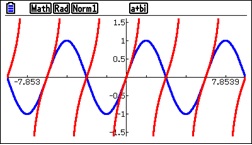
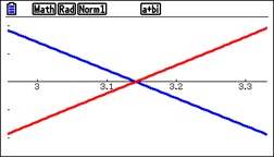
, which using the dominance idea is zero. Of course your students may try graphing or a table. Here’s the graph done by a TI-Nspire CAS. Note the scales.

This is not the way to go. Since the function is increasing near the origin, but the limit at infinity is zero there must be a maximum point where the function starts decreasing. And as the expression can never be negative once x > 1, there must be a point of inflection where the graph becomes concave up and can thereafter approach the x-axis from above as a horizontal asymptote. The maximum can be found by hand which makes for some great algebra manipulation practice:

\displaystyle \frac{d}{dx}\left( \frac{\ln \left( {{x}^{5}} \right)}{{{x}^{0.02}}} \right)=\frac{{{x}^{0.02}}\tfrac{5{{x}^{4}}}{{{x}^{5}}}-\ln \left( {{x}^{5}} \right)\left( 0.02{{x}^{-0.98}} \right)}{{{x}^{0.04}}}

\displaystyle \frac{d}{dx}\left( \frac{\ln \left( {{x}^{5}} \right)}{{{x}^{0.02}}} \right)=\frac{{{x}^{-0.98}}\left( 5-\left( 0.10 \right)\ln \left( x \right) \right)}{{{x}^{0.04}}}=\frac{50-\ln \left( x \right)}{10{{x}^{1.02}}}

Setting this equal to zero and solving gives x={{e}^{50}}\approx 5.185\times {{10}^{21}}

The second derivative is \displaystyle \frac{{{d}^{2}}}{d{{x}^{2}}}\left( \frac{\ln \left( {{x}^{5}} \right)}{{{x}^{0.02}}} \right)=\frac{-510+10.2\ln \left( x \right)}{100{{x}^{2.02}}}

and is zero when x\displaystyle {{e}^{\frac{520}{10.2}}}\approx 1.382\times {{10}^{22}}

Okay, I skipped a few steps here, but you can challenge your students with that. Since we’re really interested in the solution here more than the solving ,this is really a good place to use a CAS calculator.

The first line in the figure above defines the function to save typing it each time. The second line finds the x-coordinate of the maximum point (how do we know this is a maximum?) and the third finds the x-coordinate of the point of inflection.  Much simpler this way!

Take a minute to consider the numbers. They are BIG! In fact, if the units on our graph paper are centimeters, then the maximum point is a little over 5,480 light-years away from the origin! The point of inflection is about 2.665 times farther at more than 14,607 light-years away!

Meanwhile the maximum value is only 91.9699 cm. That’s right centimeters, less than a meter. And the y-coordinate of the point of inflection is about 91.9524 cm. A drop of 0.0175 cm. in a horizontal distance of a little over 9,127 light-years.

Some problems are a lot less scary if done with technology.


Why Radians?

Calculus is always done in radian measure. Degree (a right angle is 90 degrees) and gradian measure (a right angle is 100 grads) have their uses. Outside of the calculus they may be easier to use than radians. However, they are somewhat arbitrary. Why 90 or 100 for a right angle? Why not 10 or 217?

Radians make it possible to relate a linear measure and an angle measure. A unit circle is a circle whose radius is one unit. The one-unit radius is the same as one unit along the circumference. Wrap a number line counterclockwise around a unit circle starting with zero at (1, 0). The length of the arc subtended by the central angle becomes the radian measure of the angle.

This keeps all the important numbers like the sine and cosine of the central angle, on the same scale. When you graph y = sin(x) one unit in the x-direction is the same as one unit in the y-direction. When graphing using degrees, the vertical scale must be stretched a lot to even see that the graph goes up and down. Try graphing on a calculator y = sin(x) in degree mode in a square window and you will see what I mean.

But the utility of radian measure is even more obvious in calculus. To develop the derivative of the sine function you first work with this inequality (At the request of a reader I have added an explanation of this inequality at the end of the post):

\displaystyle \frac{1}{2}\cos \left( \theta \right)\sin \left( \theta \right)\le \frac{1}{2}\theta \le \frac{1}{2}\tan \left( \theta \right)

From this inequality you determine that \displaystyle \underset{\theta \to 0}{\mathop{\lim }}\,\frac{\sin \left( \theta \right)}{\theta }=1

The middle term of the inequality is the area of a sector of a unit circle with central angles of \theta 
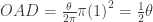
radians. If you work in degrees, this sector’s area is \displaystyle \frac{\pi }{360}\theta  and you will find that
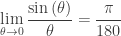
 \displaystyle \underset{\theta \to 0}{\mathop{\lim }}\,\frac{\sin \left( \theta \right)}{\theta }=\frac{\pi }{180}.

This limit is used to find the derivative of the sin(x). Thus, with x in degrees, \displaystyle \frac{d}{dx}\sin \left( x \right)=\frac{\pi }{180}\cos \left( x \right)
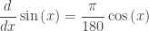
. This means that with the derivative or antiderivative of any trigonometric function that \displaystyle \frac{\pi }{180} is there getting in the way.

Who needs that?

Do your calculus in radians.


Revision December 7, 2014: The inequality above is derived this way. Consider the unit circle shown below.

unit circle

1. The central angle is \theta  and the coordinates of A are \left( \cos (\theta ),\sin (\theta ) \right).

Then the area of triangle OAB is \frac{1}{2}\cos \left( \theta\right)\sin \left( \theta\right)

2. The area of sector OAD=\frac{\theta}{2\pi }\pi {{\left( 1 \right)}^{2}}=\frac{1}{2}\theta 
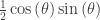
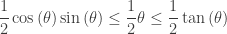
. The sector’s area is larger than the area of triangle OAB.
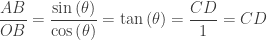
3. By similar triangles \displaystyle \frac{AB}{OB}=\frac{\sin \left( \theta\right)}{\cos \left( \theta\right)}=\tan \left( \theta\right)=\frac{CD}{1}=CD.

Then the area of \Delta OCD=\frac{1}{2}CD\cdot OD=\frac{1}{2}\tan \left( \theta \right) This is larger than the area of the sector, which establishes the inequality above.

Multiply the inequality by \displaystyle \frac{2}{\sin \left( \theta \right)} and take the reciprocal to obtain
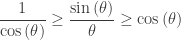
 \displaystyle \frac{1}{\cos \left( \theta \right)}\ge \frac{\sin \left( \theta \right)}{\theta }\ge \cos \left( \theta \right).

Finally, take the limit of these expression as \theta \to 0 and the limit \displaystyle \underset{\theta \to 0}{\mathop{\lim }}\,\frac{\sin \left( \theta \right)}{\theta }=1 is established by the squeeze theorem.

The Derivative II

(In this activity I am paraphrasing and expanding the suggestions of Alan Lipp in a posting “Derivatives of Trig Functions” August 29, 2012 to the Calculus Electronic Discussion Group.)

This activity parallels the one in my last post here using technology.

    1. Enter the function you are investigating as Y1 in your calculator. Later you will change this to other functions but will not have to change the following entries.  Start with Y1 = x2.
    2. Enter

      \displaystyle Y2=\frac{Y1(x+0.0001)-Y1(x)}{0.0001}.

      This will approximate the derivative. This expression is called the forward difference quotient.

    1. Graph in a square window.
    1. Guess the equation of the graph you see for Y2, enter you guess in Y3 and graph it. If your guess is correct what should you see?
    1. Deselect Y1 and produce a table for the Y2 and Y3 graph. Do the values of Y2 look like what you guessed for Y3? If not, adjust your guess for Y3. (Hint: because Y2 is an approximation, they will be close but not exact.)
  1. Another way to check your guess is to graph Y4 = Y2/Y3. If your guess is close, Y4 should be the line y = 1. If their guess is wrong, the graph of Y4 may give a clue as to the correct answer. If the guess the derivative of x2 is x, then Y4 = 2 hinting that the correct guess is 2x.

A comment: Calculators have a built in numerical derivative function usually called nDeriv or d/dx. You may use this in step 2 above. However, entering and using the expression for the approximate derivative as above, reinforces the concept and is more transparent for the student than using some strange new built-in function.

Now repeat the exercise above with other functions. Chose functions whose derivatives are easy to guess for example, y = x3, y = x4, y = x5, etc., and  y = sin(x), and y = cos(x).

Keep a list of the results, so you can check it later.