Good Question 11 – Riemann Reversed

Posted on November 29, 2016 by Lin McMullin

Good Question 11 – or not.

The question below appears in the 2016 Course and Exam Description (CED) for AP Calculus (CED, p. 54), and has caused some questions since it is not something included in most textbooks and has not appeared on recent exams. The question gives a Riemann sum and asks for the definite integral that is its limit. Another example appears in the 2016 “Practice Exam” available at your audit website; see question AB 30. This type of question asks the student to relate a definite integral to the limit of its Riemann sum. These are called reversal questions since you must work in reverse of the usual order. Since this type of question appears in both the CED examples and the practice exam, the chances of it appearing on future exams look good.

To the best of my recollection the last time a question of this type appeared on the AP Calculus exams was in 1997, when only about 7% of the students taking the exam got it correct. Considering that by random guessing about 20% should have gotten it correct, this was a difficult question. This question, the “radical 50” question, is at the end of this post.

Example 1

Which of the following integral expressions is equal to $\displaystyle \underset{n\to \infty }{\mathop{\lim }}\,\sum\limits_{k=1}^{n}{\left( \sqrt{1+\frac{3k}{n}}\cdot \frac{1}{n} \right)}$ ?

There were 4 answer choices that we will consider in a minute.

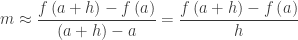
The first key to answering the question is to recognize the limit as a Riemann sum. In general, a right-side Riemann sum for the function f on the interval [a, b] with n equal subdivisions, has the form:

$\displaystyle \underset{n\to \infty }{\mathop{\lim }}\,\sum\limits_{k=1}^{n}{\left( f\left( a+\frac{b-a}{n}\cdot k \right)\cdot \frac{b-a}{n} \right)}=\int_{a}^{b}{f\left( x \right)dx}$

To evaluate the limit and express it as an integral, we must identify, a, b, and f. I usually begin by looking for $\displaystyle \frac{b-a}{n}$ . Here $\displaystyle \frac{b-a}{n}=\frac{1}{n}$ and from this conclude that b – a = 1, so b = a + 1.

Usually, you can start by considering a = 0 , which means that the $\displaystyle \frac{b-a}{n}\cdot k$ becomes the “x.”. Then rewriting the radicand as $\displaystyle 1+3\frac{1}{n}k=1+3\left( a+\frac{1}{n}\cdot k \right)$ , it appears the function is $\sqrt{1+3x}$ and the limit is $\displaystyle \int_{0}^{1}{\sqrt{1+3x}}dx=\frac{14}{9}$ .

The answer choices are

(A) $\displaystyle \int_{0}^{1}{\sqrt{1+3x}}dx$ (B) $\displaystyle \int_{0}^{3}{\sqrt{1+x}}dx$ (C) $\displaystyle \int_{1}^{4}{\sqrt{x}}dx$ (D) $\displaystyle \tfrac{1}{3}\int_{0}^{3}{\sqrt{x}}dx$

The correct choice is (A), but notice that choices B, C, and D can be eliminated as soon as we determine that b = a + 1. That is not always the case.

Let’s consider another example:

Example 2: $\displaystyle \underset{n\to \infty }{\mathop{\lim }}\,\sum\limits_{k=1}^{n}{\left( {{\left( 2+\frac{3}{n}k \right)}^{2}}\left( \frac{3}{n} \right) \right)}=$

As before consider $\displaystyle \frac{b-a}{n}=\frac{3}{n}$ , which implies that b = a + 3. With a = 0, the function appears to be ${{\left( 2+x \right)}^{2}}$ on the interval [0, 3], so the limit is $\displaystyle \int_{0}^{3}{{{\left( 2+x \right)}^{2}}}dx=39$

BUT

What if we take a = 2? If so, the limit is $\displaystyle \int_{2}^{5}{{{x}^{2}}dx}=39$ .

And now one of the “problems” with this kind of question appears: the answer written as a definite integral is not unique!

Not only are there two answers, but there are many more possible answers. These two answers are horizontal translations of each other, and many other translations are possible, such as $\displaystyle \int_{-25.65}^{-22.65}{{{\left( 27.65+x \right)}^{2}}dx}=39$ .

The same thing can occur in other ways. Returning to example 1,and using something like a u-substitution, we can rewrite the original limit as $\displaystyle \frac{1}{3}\cdot \underset{n\to \infty }{\mathop{\lim }}\,\sum\limits_{k=1}^{n}{\left( \sqrt{1+\frac{3k}{n}}\cdot \frac{3}{n} \right)}$ .

Now b = a + 3 and the limit could be either $\displaystyle \frac{1}{3}\int_{0}^{3}{\sqrt{1+x}}dx=\frac{14}{9}$ or $\displaystyle \frac{1}{3}\int_{1}^{4}{\sqrt{x}}dx=\frac{14}{9}$ , among others.

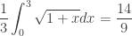
My opinions about this kind of question.

The real problem with the answer choices to Example 1 is that they force the student to do the question in a way that gets one of the answers. It is perfectly reasonable for the student to approach the problem a different way, and get a different correct answer that is not among the choices. This is not good.

The problem could be fixed by giving the answer choices as numbers. These are the numerical values of the 4 choices:(A) 14/9 (B) 14/3 (C) 14/3 (D) $2\sqrt{3}/3$ . As you can see that presents another problem. Distractors (wrong answers) are made by making predictable calculus mistakes. Apparently, two predictable mistakes give the same numerical answer; therefore, one of them must go.

A related problem is this: The limit of a Riemann sum is a number; a definite integral is a number. Therefore, any definite integral, even one totally unrelated to the Riemann sum, which has the correct numerical value, is a correct answer.

I’m not sure if this type of question has any practical or real-world use. Certainly, setting up a Riemann sum is important and necessary to solve a variety of problems. After all, behind every definite integral there is a Riemann sum. But starting with a Riemann sum and finding the function and interval does not seem to me to be of practical use.

The CED references this question to MPAC 1: Reasoning with definitions and theorems, and to MPAC 5: Building notational fluency. They are appropriate,and the questions do make students unpack the notation.

My opinions notwithstanding, it appears that future exams will include questions like these.

These questions are easy enough to make up. You will probably have your students write Riemann sums with a small value of n when you are teaching Riemann sums leading up to the Fundamental Theorem of Calculus. You can make up problems like these by stopping after you get to the limit, giving your students just the limit, and having them work backwards to identify the function(s) and interval(s). You could also give them an integral and ask for the associated Riemann sum. Question writers call questions like these reversal questions since the work is done in reverse of the usual way.

Here is the question from 1997, for you to try. The answer is below.

Answer B. Hint n = 50

Revised 5-5-2022

From One Side or the Other.

Posted on November 1, 2016 by Lin McMullin

Recently, a reader wrote and suggested my post on continuity would be improved if I discussed one-sided continuity. This, along with one-sided differentiability, is today’s topic.

The definition of continuity requires that for a function to be continuous at a value x = a in its domain $\underset{x\to a}{\mathop{\lim }}\,f\left( x \right)=f\left( a \right)$ and that both values are finite. That is, the limit as you approach the point in question be equal to the value at that point. This limit is a two-sided limit meaning that the limit is the same as x approaches a from both sides. That definition is extended to open intervals, by requiring that for a function to be continuous on an open interval, that it is continuous at every point of the interval

How do you check every point? One way is to prove the limit in the definition in general for any point in the open interval. Another is to develop a list of theorems that allow you to do this. For example, f(x) = x can be shown to be continuous at every number. Then sums, differences, and products, of this function allows you to extend the property to polynomials and then other functions.

But what about a function that has a domain that is not the entire number line? Something like $f\left( x \right)=\sqrt{4-{{x}^{2}}},-2\le x\le 2$ . Here, $f\left( -2 \right)=f\left( 2 \right)=0$ ; the function is defined at the endpoints. A look at the graph shows a semi-circle that appears to contain the endpoints (–2, 0) and (2, 0). The function is continuous on the open interval (–2, 2) but cannot be continuous under the regular definition since the limit at the endpoints does not exist. The limit does not exist because the limit from the left at the left-endpoint, and the limit from the right at the right endpoint do not exist. What to do?

What is done is to require only that the one-sides limits from inside the domain exist. Here they do: $\underset{x\to -2+}{\mathop{\lim }}\,f\left( x \right)=0$ and the $\underset{x\to 2-}{\mathop{\lim }}\,f\left( x \right)=0$ and since the limits equal the values we say the function is continuous on the closed interval [–2, 2]. In general, when you say a function is continuous on a closed interval, you mean that the one-sided limits from inside the interval exist and equal the endpoint values.

You can determine that the limits exist by finding them as in the example above. Another way is to realize that if a < b < c < d and the function is continuous on the open (or closed) (a, d) then it is continuous on the closed interval [b c].

Why bother?

The reason we take this trouble is because for some reason the proof of the theorem under consideration requires that the endpoint value not only exist but hooks up with the function to make it continuous. Thus, the continuity on a closed interval is included in the hypotheses of theorem where this property is required. For example, the Intermediate Value Theorem would not work on a function that had no endpoints for $f\left( c \right)$ to be between. Also, the Mean Value Theorem requires you to find the slope between the endpoints, so the endpoint needs to be not only defined, but attached to the rest of the function.

One-sided differentiability

The definition of the derivative at a point also requires a two-sided limit to exist at the point. Most of the early theorems in calculus require only that the function be differentiable on an open interval.

Is it possible to define differentiability at the endpoint of an interval? Yes. It’s done in the same way by using a one-sided limit. If x = a is the left endpoint of an interval, then the derivative from the right at that point is defined as

$\displaystyle {f}'\left( a \right)=\underset{h\to 0+}{\mathop{\lim }}\,\frac{f\left( a+h \right)-f\left( a \right)}{h}$ .

By letting h approach 0 only from the right, you never consider values outside the interval. (At the right endpoint a similar definition is used with $h\to 0-$ ).

So why don’t we ever see one-sided derivatives? Because the theorems do not need them to prove their result. Hypotheses of theorems should be the minimum requirements needed, so if there is no need for the function to be differentiable at an endpoint, this is not listed in the hypotheses. This makes the hypothesis less restrictive and, therefore, covers more situations.

One theorem, beyond what is usually covered in beginning calculus, where endpoint differentiability is needed is Darboux’s Theorem. Darboux’s Theorem is sometime called the Intermediate Value Theorem for derivatives. It says that the derivative takes on all values between the derivatives at the endpoints, and thus needs the one-sided derivatives at the endpoints to exist. Interestingly, Darboux’s Theorem does not require the function to be continuous on the open interval between the endpoints.

Continuous Fun

Posted on October 13, 2015 by Lin McMullin

The topic of this post is continuity. The phrase “a function is continuous on its domain” was much discussed last week on the AP Calculus Community bulletin board as it is about this time every year. This led to a discussion of one-sided continuity at the endpoint of an interval.

Let’s start by looking at some definitions related to continuity. A detailed discussion of definitions is worth doing in any math class; it helps students learn about the structure of mathematics. Definitions are biconditional statements; that is, either part implies the other.

Definitions related to Continuity

A function is continuous at a point, (a, f(a)) if, and only if, (1) f(a) exists (is a finite number), and (2) $\displaystyle \underset{x\to a}{\mathop{\lim }}\,f\left( x \right)$ exists (is a finite number), and (3) $\displaystyle \underset{x\to a}{\mathop{\lim }}\,f\left( x \right)=f\left( a \right)$ – the limit equals the value.

This is the three-part definition you will find in most textbooks. The first two conditions are sort of for emphasis since the third is not possible if the limit does not exist (or is infinite) and/or the value does not exist (DNE). Graphically this means that as you move along the graph of f getting closer to the place where x = a the function values are getting closer to f(a). This is not always the case; specifically, if this does not happen the function is not continuous at the point.

For example, let $\displaystyle f\left( x \right)=\frac{x-3}{(x-2)(x-3)}$

This function is undefined at x = 2 and x = 3; at both values f(x) DNE.
At x = 3 the limit does exist and is equal to 1. In this case the graph appears to be missing a single point, here (3, 1). This is called a removable discontinuity because be redefining the function so that f(3) = 1 the function could be made continuous. This happens most often when the factor in the denominator that becomes zero “cancels” with a like factor in the numerator. This can also happen if the function value is defined as something different than the limit. There are other examples such as $\displaystyle \frac{\sin \left( x \right)}{x}$ at x = 0
At x = 2 the limit DNE, and the situation appears as a vertical asymptote on the graph: on the left the values approach negative infinity and on the right they approach positive infinity. This is because a factor in the denominator gets very small as you approach 2.

Proving a function is continuous has been asked on AP Calculus exams. (See 2003 AB 6a and 2011 AB 6a) Students were expected to state the value of the two one-sided limits and the value of the function to show the three parts of the definition were true.

A function is continuous on an open interval if, and only if, it is continuous at every point in the interval.

The definition of continuous at a point is extended to all the points of an interval. But do you have to check each and every point? No, this is determined by finding where the function is not continuous; the function is then continuous on the intervals between these points.

In many theorems it is necessary to have a function be continuous on a closed interval; the endpoints must be included, but the limit in the main definition is a two-sided limit. The main definition is adapted to read A function is continuous from the right at x = a (or from the left at x = b) if, and only if, $\displaystyle \underset{x\to a+}{\mathop{\lim }}\,f\left( x \right)=f\left( a \right)\text{ }\left( \underset{x\to b-}{\mathop{\lim }}\,f\left( x \right)=f\left( b \right) \right)$ .

The limits are approached from inside the interval: from the right at the left end and from the left at the right end.

Continuous on its Domain

Functions exist only on their domain, so there is no way a function can be continuous except on its domain. I wrote about this is a previous post Right answer, Wrong Question.

When analyzing a new function one of the things you look for is where the function is continuous. But really you do this by looking for places where it is not continuous; everywhere else the function will be continuous.

Vertical asymptotes, removable discontinuities, and oscillating discontinuities are not possible for a function continuous on its domain; these appear on the graph, but mark places where the function DNE. The only kind of discontinuity a function may have on its domain are jump or step discontinuities. These often occur with piecewise defined functions where the endpoint of one piece is defined and different from the corresponding endpoint of the next piece. For example,

$\displaystyle f\left( x \right)=\left\{ \begin{matrix} \sin \left( x \right) & 0\le x\le \pi \\ \cos \left( x \right) & \pi <x\le 2\pi \\ \end{matrix} \right.$

Since $f\left( \pi \right)=0$ the function is defined there, but the limits of the two parts (0 and -1) are not the same, so the function is defined, but not continuous on its domain.

Another example is the greatest integer function (aka the floor function) whose graph is shown in below. Note that the left-endpoint of each segment (at the integer values) is included, while the right-endpoint at the next integer is not included.

Spotting discontinuities

Here are some hints on looking for places where a function is not continuous:

Look for the zeros of the denominators
For piecewise functions check the places where the pieces change definition.
For trigonometric functions, the sine and cosine are continuous for all x. Since the other trigonometric functions are defined in terms of the sine and cosine look places where the sine or cosine is zero and appears in the denominator of the definition.
Function involving square roots and other even degree roots are not defined, and therefore not continuous where their arguments are negative. For example, $\sqrt{4-{{x}^{2}}}$ is continuous on the closed interval [-2, 2] (using the definitions for closed intervals – one-sided limits), but not elsewhere.
Use technology to graph the function; discontinuities usually show up. The exception is a removable discontinuity or an oscillating discontinuity which may not show up because the x-value of the discontinuity may not be a pixel coordinate.

Pathological Examples

This function, attributed to Dirichlet, is defined for all Real numbers, but not continuous anywhere.

$f\left( x \right)=\left\{ \begin{matrix} 1 & \text{if }x\text{ is irrational} \\ 0 & \text{if }x\text{ is rational} \\ \end{matrix} \right.$

Between every pair of irrational numbers is a rational number, and between every pair of rational numbers is an irrational number.

With a slight variation, we have this function:

$\displaystyle g\left( x \right)=\left\{ \begin{matrix} 1 & \text{if }x\text{ is irrational} \\ x & \text{if }x\text{ is rational} \\ \end{matrix} \right.$

This function is defined for all Real numbers and is continuous at only one point (1, 1). Go figure.

Determining the Indeterminate

Posted on September 24, 2015 by Lin McMullin

When determining the limit of an expression the first step is to substitute the value the independent variable approaches into the expression. If a real number results, you are all set; that number is the limit.

When you do not get a real number often expression is one of the several indeterminate forms listed below:

Indeterminate Forms:

$\displaystyle \frac{0}{0},\quad \quad \frac{\pm \infty }{\pm \infty },\quad \quad 0\cdot \infty ,\quad \quad \infty -\infty ,\quad \quad {{0}^{0}},\quad \quad {{1}^{\infty }},\quad \quad {{\infty }^{0}}$

They are called indeterminate forms because by doing some algebraic manipulation to simplify (or sometimes complicate) the expression its value can be determined. The calculus technique called L’Hôpital’s Rule may be used in some situations.

Part of the reason they are called indeterminate forms is that different expressions with the same indeterminate form may result in different values.

Before continuing with the discussion of indeterminate forms, I should point out that there are also determinate forms: expressions similar to those above that always result in the same value.

Determinate Forms and the values they approach:

$\displaystyle \frac{1}{\pm \infty }\to 0,\quad \infty +\infty \to \infty ,\quad \infty \cdot \infty \to \infty ,\quad {{0}^{\infty }}\to 0,\quad \frac{1}{{{0}^{\infty }}}={{0}^{-\infty }}\to \infty$

Returning to indeterminate forms, textbooks contain examples and exercises that illustrate how to evaluate the indeterminate forms. Here are two examples illustrating a few of the techniques that can be used to evaluate them.

Example 1: $\displaystyle \underset{x\to \infty }{\mathop{\lim }}\,{{\left( 1+\frac{1}{x} \right)}^{x}}=?$ .This is an example of the indeterminate form ${{1}^{\infty }}$ . With exponents, logarithms may often be used to find the value.

The limit is now of the indeterminate form $\frac{0}{0}$ , so L’Hôpital’s Rule may be used. Continuing

$\displaystyle \ln \left( ? \right)=\underset{x\to \infty }{\mathop{\lim }}\,\left( x\ln \left( 1+\frac{1}{x} \right) \right)=\underset{x\to \infty }{\mathop{\lim }}\,\frac{\ln \left( 1+\frac{1}{x} \right)}{\frac{1}{x}}=\underset{x\to \infty }{\mathop{\lim }}\,\frac{\left( \frac{1}{1+\frac{1}{x}} \right)\left( -{{x}^{-2}} \right)}{-{{x}^{-2}}}=\underset{x\to \infty }{\mathop{\lim }}\,\left( \frac{1}{1+\frac{1}{x}} \right)=1$

So then ln(?) = 1 and ? = e¹ = e and therefore $\displaystyle \underset{x\to \infty }{\mathop{\lim }}\,{{\left( 1+\frac{1}{x} \right)}^{x}}=e$

Example 2: $\displaystyle \underset{x\to 0}{\mathop{\lim }}\,\left( \frac{\sin \left( x+\frac{\pi }{6} \right)}{x}-\frac{\sin \left( \frac{\pi }{6} \right)}{x} \right)$ is an example of the indeterminate form $\infty -\infty$ .

Write the expression with a common denominator:

$\displaystyle \underset{x\to 0}{\mathop{\lim }}\,\left( \frac{\sin \left( x+\frac{\pi }{6} \right)}{x}-\frac{\sin \left( \frac{\pi }{6} \right)}{x} \right)=\underset{x\to 0}{\mathop{\lim }}\,\left( \frac{\sin \left( \frac{\pi }{6}+x \right)-\sin \left( \frac{\pi }{6} \right)}{x} \right)=\cos \left( \frac{\pi }{6} \right)=\frac{\sqrt{3}}{2}$

The second limit above is the definition of the derivative of $\sin \left( \frac{\pi }{6} \right)$ . (L’Hôpital’s Rule may also be used with the second limit above.)

In fact, the definition of the derivative of all (any, every) functions, $\displaystyle {f}'\left( a \right)=\underset{h\to 0}{\mathop{\lim }}\,\frac{f\left( a+h \right)-f\left( a \right)}{h}$ , gives indeterminate expressions of the form $\frac{0}{0}$ .

Discovering the Derivative

Posted on August 18, 2015 by Lin McMullin

Discovering the Derivative with a Graphing Calculator

This is an outline of how to introduce the idea that the slope of the line tangent to a graph can be found, or at least approximated, by finding the slope of a line through two very close points in the graph. It is a set of graphing calculator activities that will use graphs and numbers to lead to the symbolic form of the derivative.

You may work through the activities with your class (which is what I would do) or you could write and distribute them and let your class do them a laboratory exercise. Before starting students should know how to use their calculator to graph, to trace to points on the graph, and how to save and recall the coordinates from the graph to variables on the home screen using the graphing calculator’s store feature.

I suggest you work through these three times (or more) using different functions. I will work with $y={{x}^{2}}$ . A good second example is $y={{x}^{3}}$ , and a third example to use is $y=\sin \left( x \right)$ . Use simple functions, because you will want the students to see the answers without too much trouble.The procedure is the same for all.

Part 1:

Begin by asking students to enter $y={{x}^{2}}$ in their calculator asY1 and graph it in a standard, square window. (Do not use the decimal window as “nice” decimals are not necessary or helpful.)
Figure 1
Next, have them trace over to different points on the graph (some should go left and others to the right); they should all end up at different points. Then have them zoom-in 6 or 8 times until the graph looks linear. (This is local linearity – functions that are differentiable are locally linear.)
Then push TRACE to be sure the cursor is on the graph. The coordinates of the point are on the bottom of the screen. Go to the HOME screen and save the two values as a and b. Think of this first point as (a, b).
Return to the graph screen and push TRACE. This should return the cursor to the first point. (If not, close is okay.) Then click to the right or to left once, or twice at most, to move to a nearby point on the graph. Return to the home screen and save the new values to c and d for the second point (c, d).
On the home screen use a, b, c, and d to write the slope of the line through the two points. See figure 1. (Go around the room as they are doing this and make sure students are getting this – their slope should be approximately twice a or c.)
Return to the equation screen and enter the equation of the line through the two points asY2. (See figure 2). Graph this equation with the parabola.
Figure 2
Have the students record their values of a, b, c, d and m on paper (three decimal places will be enough) and also write a description of what they see on the graph and why they think this is so. (This is in case they lose the numbers on their calculator when they do another graph and also because you will need them later in the next part of the exploration.)

Repeat the same steps separately with the other two functions and record the results in the same way. Write their numbers and observations. Discuss the observations with the class.

Of course, the lines should look tangent to the graphs, but since they contain two points of the graph, they cannot actually be tangent.
Discuss how a line can be tangent to a graph. How is this different from a tangent to a circle?
Ask what could be done to make their line even closer to being tangent. (Use points closer together.)

Part 2:

Now you have homework to do. Collect the student’s data and combine it into a list with columns for a, c, and m. The points do not have to be in order. Leave any “wrong” points for discussion; if there are none, you might want to make one up and include it. Do this for each of the three sets of data. Make a copy for each student. Enter the numbers for a and m as lists in your emulator and make a dot-plot of the points (a, m) = (a, slope at x = a).

Return the lists of points to the students and ask them to study the list and see if they can see any obvious relationship between the numbers on each line. Answers for y = x² should be the m is approximately twice either a or c; or maybe some will see that m is approximately a + c. Answers for y = x³ will be less obvious (three times the square of a). Answers for y = sin(x) will not be obvious at all.
Using the emulator, separately for each of the three sets of data, make a dot-plot of the numbers (use a square window). Ask the student to discuss what they see. See if they can find an equation of the graph of the dot-plots. Now the equation of the data set for sin(x) should be obvious. Plot their guesses on top of the points and see how close they come.

Part 3:

Now guide the class through the symbolic explanation of what they did. Ask them to explain and write in symbols specifically what they did. The idea here is for you, the teacher, to ask lots of leading questions until the class decides on the best answer.

Call the first point (a, f(a)). Let h = “a little bit.” then the second is the point (a plus a little bit, f(a plus a little bit)) or (a + h, f(a + h)). Recall that h may have been negative for some students so the second point may actually be to the left of the first. Then help them come up with

$\displaystyle m\approx \frac{f\left( a+h \right)-f\left( a \right)}{\left( a+h \right)-a}=\frac{f\left( a+h \right)-f\left( a \right)}{h}$

Or they may prefer

$\displaystyle m\approx \frac{f\left( a \right)-f\left( c \right)}{a-c}$

Ask how this could be made “less approximate” and more actually equal. (Answer: smaller and smaller value of h.) Ask them to find the value of h = a – c for their points. How small are they? How can you make them really small? (Find a limit.)
Notice that h cannot be zero in these expressions. Keep hinting until someone comes up with the idea of finding

$\displaystyle \underset{h\to 0}{\mathop{\lim }}\,\frac{f\left( a+h \right)-f\left( a \right)}{h}$ or $\displaystyle \underset{a\to c}{\mathop{\lim }}\,\frac{f\left( a \right)-f\left( c \right)}{a-c}$

Next have the students calculate the limits below by actually doing the algebra. (They will not be able to handle the sin(x) at this point so save that for later.)

$\displaystyle \underset{h\to 0}{\mathop{\lim }}\,\frac{{{\left( x+h \right)}^{2}}-{{\left( x \right)}^{2}}}{h}\text{ and }\underset{h\to 0}{\mathop{\lim }}\,\frac{{{\left( x+h \right)}^{3}}-{{\left( x \right)}^{3}}}{h}$

Compare the answers here with the earlier work and guesses, and discuss.

… And now you are ready to define the limits as the f ’(a) derivative of f at x = a.

Good Question 5: 1998 AB2/BC2

Posted on July 29, 2015 by Lin McMullin

Continuing my occasional series of some of my favorite teaching questions, today we look at the 1998 AP Calculus exam question 2. This question appeared on both the AB and BC exams. I use this problem to illustrate two very different questions that come up almost every time I lead a workshop or an AP Summer Institute. The first is if a limit is infinite, should you say “infinite” or “does not exist (DNE)”? The second is if the student solves the problems correctly, but by some other method, maybe even one not using the calculus, do they still earn full credit? In addition to discussing these two questions I’ll have a few suggestions for how to use this kind of question for teaching (maybe in other than a calculus class).

The question had the student examine the function $f\left( x \right)=2x{{e}^{2x}}$ and, although it is easy enough to answer without, students were allowed to use their graphing calculator. A reasonable student probably looked at a graph of the function.

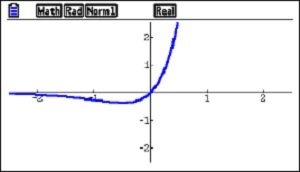
$f\left( x \right)=2x{{e}^{2x}}$

Part a: First the question asks the student to explore the end behavior of the function by finding two limits: $\underset{x\to -\,\infty }{\mathop{\lim }}\,f\left( x \right)$ and $\underset{x\to \infty }{\mathop{\lim }}\,f\left( x \right)$ . The students should not depend on the graph here. As $x\to -\infty$ , ${{e}^{2x}}$ approaches zero and since the exponential function dominates the polynomial, $\underset{x\to -\,\infty }{\mathop{\lim }}\,f\left( x \right)=0$ . In passing note that for x < 0 the function is negative and approaches zero from below. No work or explanation was required, but when teaching things like this be sure students know and can explain their answer without reference to their calculator graph. For the second limit, since both factors increase without bound $\underset{x\to \infty }{\mathop{\lim }}\,f\left( x \right)=\infty$ If the student wrote $\underset{x\to \infty }{\mathop{\lim }}\,f\left( x \right)=\text{DNE}$ , he received full credit.

Infinity is not a number, so there really is no limit in the second case; the limit DNE. But there are other ways a limit may not exist such as a jump discontinuity or an oscillating discontinuity. DNE covers these as well as infinite limits. Saying a limit is infinite tells us more about the limit than DNE. It tells us that the function increases without bound; that eventually it becomes greater than any number.

Both answers are correct.

But we’re not done with this yet. We will come back to it before the question is done.

Part b: Students were asked to find and justify the minimum value of the function. Using the first derivative test, students proceeded by finding where the derivative is zero..

${f}'\left( x \right)=\left( 2x \right)\left( 2{{e}^{2x}} \right)+2{{e}^{2x}}=2{{e}^{2x}}\left( 2x+1 \right)=0$

$x=-\frac{1}{2}$

$f\left( -\tfrac{1}{2} \right)=2\left( -\tfrac{1}{2} \right){{e}^{2\left( -\tfrac{1}{2} \right)}}=-\frac{1}{e}\approx 0.368\text{ or }0.367$

Justification: If $x<-\tfrac{1}{2},\ {f}'\left( x \right)<0$ and if $x>-\tfrac{1}{2},\ {f}'\left( x \right)>0$ , therefore the absolute minimum is $-\frac{1}{e}$ and occurs at $x=-\frac{1}{2}$ .

All pretty straightforward

Part c: This part asked for the range of the function. Here the student must show that if he wrote DNE in part a, he knows that in fact the function grows without bound.

Putting together the answers from part a and part c, the range is $f\left( x \right)\ge -\frac{1}{e}$ , which may also be written as $\left[ -1/e,\infty\right)$ . (The decimals could also be used here.)

Part d: asked students to consider functions given by $y=bx{{e}^{bx}}$ where b was a non-zero number. The question required students to show that the absolute minimum value of all these functions was the same.

Most students did what was expected and preceded as in part b. The work is exactly the same as above except that all of the 2s become bs. The absolute minimum occurs at $x=-\frac{1}{b}$ and $y\left( -\tfrac{1}{b} \right)=-\frac{1}{e}$ .

BUT ….

Other students found a way completely without “calculus.” Can you find do that?

They realized that the given function as a horizontal expansion or compression, possibly including a reflection over the y-axis, of and therefore the range is the same for all these functions and so the minimum value must be the same. This received full credit. The rule of thumb is “don’t take off for good mathematics.”

Pretty cool!

The graphs of several cases are shown below

$y=bx{{e}^{bx}}$
b = -5 in blue, b = -1 in red, b = 2 in green, and b = 4 in magenta.

Teaching Suggestions

I can see using this in a pre-calculus class. The calculus (finding the minimum for b = 2 or in general) is straightforward. In a pre-calculus setting as an example of transformations it may be more useful. You could give students 6, or 8, or 10 examples with different values of b, both positive and negative.

First ask students to investigate the end behavior by finding the limits as x approaches positive and negative infinity. The results will be similar. Have them write a summary considering two cases: b > 0 and b < 0.
Graphing calculators have built-in operations that will find the x-coordinates or both coordinates of the minimum point of a function. Since we’re concerned with the transformation and not the calculus, let students use their graphing calculators to find the coordinates of the minimum point of each graph (as decimals). See if they can determine the x-coordinate in terms of b. They should also notice that y-coordinates will all be the same (about -0.367880).
Finally, set the class to proving using their knowledge of transformation that the minimums are really all the same.

Good Question 1: 2008 AB 6

Posted on January 21, 2015 by Lin McMullin

When I started this blog several years ago I was hoping my readers would ask questions that we could discuss or submit ideas for additional topics to write about. This has not really happened, but I’m still very open to the idea. (That was a HINT.) Since that first year when I had the entire curriculum ahead of me, I have written less not because I dislike writing, but because I am low on ideas.

The other day, I answered a question posted on the AP Calculus Community bulletin board about AB calculus exam question. It occurred to me that this somewhat innocuous looking question was quite good. So I decided to start an occasional series on good questions, from AP exams or elsewhere, that can be used to teaching beyond the actual things asked in the question. (My last post might be in this category, but that was written several months ago.)

In discussing these questions, I will make numerous comments about the question and how to take it further in your class. My idea is not just to show how to write a good answer, but rather to use the question to look deeper into the concepts involved.

Good Question #1: 2008 AB Calculus exam question 6.

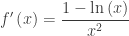
The stem gave students the function $\displaystyle f\left( x \right)=\frac{\ln \left( x \right)}{x},\quad x>0$ . Students were also told that $\displaystyle {f}'\left( x \right)=\frac{1-\ln \left( x \right)}{{{x}^{2}}}$ .

The first thought that occurs is why they gave the derivative. The reason is, as we will see, that the first derivative is necessary to answer the first three parts of the question. Therefore, a student who calculates an incorrect derivative is going to be in big trouble (and the readers may have a great deal of work to do reading with the student’s incorrect work). The derivative is calculated using the quotient rule, and students will have to demonstrate their knowledge of the quotient rule later in this question; there is no reason to ask them to do the same thing twice.
If you are using this with a class, you can, and probably should, ask your students to calculate the first derivative. Then you can see how many giving the derivative would have helped.
When discussing the stem, you should also discuss the domain, x > 0, and the x-intercept (1, 0). Other features of the graph, such as end behavior, are developed later in the question, so they may be put on hold briefly.

Part a asked students to write an equation of the tangent line at x = e². To do this students need to do two calculations: $\displaystyle f\left( {{e}^{2}} \right)=\frac{2}{{{e}^{2}}}$ and $\displaystyle {f}'\left( {{e}^{2}} \right)=-\frac{1}{{{e}^{4}}}$ . An equation of the tangent line is $\displaystyle y=\frac{2}{{{e}^{2}}}-\frac{1}{{{e}^{4}}}\left( x-{{e}^{2}} \right)$ .

Writing the equation of a tangent line is a very important skill and should be straightforward. The point-slope form is the way to go. Avoid slope-intercept.
The tangent line is used to approximate the value of the function near the point of tangency; you can throw in an approximation computation here.
After doing part c, you should return here and discuss whether the approximation is an overestimate or an underestimate and how you can tell. (Answer: underestimate, since the graph is concave up here.)
After doing part c, you can also ask them to write the tangent line at the point of inflection and whether approximations near the point of inflection are overestimates or an underestimates, and why. (Answer: Since the concavity change here, it depends on which side of the point of inflection the approximation is made. To the left is an overestimate; to the right is an underestimate.)

Part b asked students to find the x-coordinate of the critical point, determine whether it is a maximum, a minimum, or neither, and to “justify your answer.” To earn credit students had to write the equation $\displaystyle {f}'\left( x \right)=0$ and solve it getting x = e. They had to state that this is a maximum because “ ${f}'\left( x \right)$ changes from positive to negative at x = e.”

This is a very standard AP exam question. To expand it in your class:

Discuss how you know the derivative changes sign here. This will get you into the properties of the natural logarithm function.
Discuss why the change in sign tells you this is a maximum. (A positive derivative indicates an increasing function, etc.)
After doing part c, you can return here and try the second derivative test.
The question asks for “the” critical point, hinting that there is only one. Students should learn to pick up on hints like this and be careful if their computation produces more or less than one.
At this point we have also determined that the function is increasing on the interval $\left( -\infty ,e \right]$ and decreasing everywhere else. The question does not ever ask this, but in class this is worth discussing as important features of the graph. On why these are half-open intervals look here.

Part c told students there was exactly one point of inflection and asked them to find its x-coordinate. To do this they had to use the quotient rule to find that $\displaystyle {{f}'}'\left( x \right)=\frac{-3+2\ln \left( x \right)}{{{x}^{3}}}$ , set this equal to zero and find the x-coordinate to be x = e^3/2.

The question did not require any justification for this answer. In class you should discuss what a justification would look like. The reason is that the second derivative changes sign here. So now you need to discuss how you know this.
Also, you can now determine that the function is concave down on the interval $\left( -\infty ,{{e}^{3/2}} \right)$ and concave up on the interval $\left({{e}^{3/2}},\infty \right)$ . Ask your class to justify this.

Part d asked student to find $\displaystyle \underset{x\to 0+}{\mathop{\lim }}\,\frac{\ln \left( x \right)}{x}$ . The answer is $-\infty$ . While this seems almost like a throwaway tacked on the end because they needed another point, it is the reason I like this question.

The question is easily solved: $\displaystyle \underset{x\to 0+}{\mathop{\lim }}\,\frac{\ln \left( x \right)}{x}=\underset{x\to 0+}{\mathop{\lim }}\,\frac{1}{x}\cdot \underset{x\to 0+}{\mathop{\lim }}\,\ln \left( x \right)=\left( \infty \right)\left( -\infty \right)=-\infty$ .
While tempting, the limit cannot be found by L’Hôpital’s Rule, because on substitution you get $\frac{-\infty }{0}$ ,which is not one of the forms that L’Hôpital’s Rule can handle.
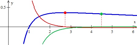
The reason I like this part so much is that we have already developed enough information in the course of doing the problem to find this limit! The function is increasing and concave down on the interval $\left( -\infty ,e \right)$ . Moving from the maximum to the left, the function crosses the x-axis at (1, 0), keeps heading south, and gets steeper. So the limit as you approach the y-axis from the right is negative infinity.This is the left-side end behavior.
What about the right-side end behavior? (You ask your class.) Well, the function is positive and decreasing to the right of the maximum and becomes concave up after x = e^3/2. Thus, it must flatten out and approach the x-axis as an asymptote.
That $\displaystyle \underset{x\to \infty }{\mathop{\lim }}\,\frac{\ln \left( x \right)}{x}=0$ is clear from the note immediately above. This limit can be found by L’Hôpital’s Rule since it is an indeterminate of the type $\infty /\infty$ . So, $\displaystyle \underset{x\to \infty }{\mathop{\lim }}\,\frac{\ln \left( x \right)}{x}=\underset{x\to \infty }{\mathop{\lim }}\,\frac{\tfrac{1}{x}}{1}=0$ .
Notice also that the first derivative approaches zero as x approaches infinity. This indicates that the function’s graph approaches the horizontal as you travel farther to the right. The second derivative also approaches zero as x approaches infinity indicating that the function’s graph is becoming flatter (less concave).

This question and the discussion is largely done analytically (working with equations). We did find a few important numbers in the course of the work. Hopefully, you students discussed this with many good words. To complete the Rule of Four, here is the graph.

And here is a close up showing the important features of the graph and the corresponding points on the derivatives.

The function is shown in blue, the derivative and maximum in red, and the second derivative and the point of inflection in green.

Finally, this function and the limit at infinity is similar to the more pathological example discussed in the post of October 31, 2012 entitled Far Out!

Teaching Calculus

The pleasure lies not in discovering the truth, but in searching for it.

Category Archives: Limits

Good Question 11 – Riemann Reversed

From One Side or the Other.

Continuous Fun

Determining the Indeterminate

Discovering the Derivative

Discovering the Derivative with a Graphing Calculator

Good Question 5: 1998 AB2/BC2

Good Question 1: 2008 AB 6

Share this:

Share this:

Share this:

Share this:

Discovering the Derivative with a Graphing Calculator

Share this:

Share this:

Share this: