
AP Type Questions 1
These questions are often in context with a lot of words describing a situation in which some things are changing. There are usually two rates given acting in opposite ways. Students are asked about the change that the rates produce over some time interval either separately or together.
The rates are often fairly complicated functions. If they are on the calculator allowed section, students should store them in the equation editor of their calculator and use their calculator to do any integration or differentiation that may be necessary.
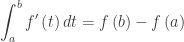
The integral of a rate of change is the net amount of change
over the time interval [a, b]. If the question asked for an amount, look around for a rate to integrate.
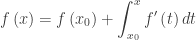
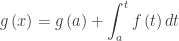
The final accumulated amount is the initial amount plus the accumulated change:
where 

What students should be able to do:
- Be ready to read and apply; often these problems contain a lot of writing which needs to be carefully read.
- Recognize that rate = derivative.
- Recognize a rate from the units given without the words “rate” or “derivative.”
- Find the change in an amount by integrating the rate. The integral of a rate of change gives the amount of change (FTC):
- Find the final amount by adding the initial amount to the amount found by integrating the rate. If
is the initial time, and
- Understand the question. It is often not necessary to as much computation as it seems at first.
- Use FTC to differentiate a function defined by an integral.
- Explain the meaning of a derivative or its value in terms of the context of the problem.
- Explain the meaning of a definite integral or its value in terms of the context of the problem. The explanation should contain (1) what it represents, (2) its units, and (3) how the limits of integration apply in context.
- Store functions in their calculator recall them to do computations on their calculator.
- If the rates are given in a table, be ready to approximate an integral using a Riemann sum or by trapezoids.
- Do a max/min or increasing/decreasing analysis.
Shorter questions on this concept appear in the multiple-choice sections. As always, look over as many questions of this kind from past exams as you can find.
For some previous posts on this subject see January 21, 23, 2013
 then
then  and
and  .
. so its inverse will contain points of the form
  , which, since we like the first coordinate of functions to be x, we may also call
  , where ln(x) will be the name of the inverse of ex. Remember, at the moment ln(x) is just a notation for the inverse of ex, we do not know anything about logarithms (yet).
 . For example, (0, 1) is a point on eX, so (1, 0) is a point on the ln(x) function, and so ln(1) = 0.
 . Now, at
  . That is


 and the t-axis between 1 and x. If
  , then
  and if
  ,
,  .
.

 ,
,  and since ln(a) is a constant
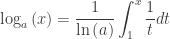
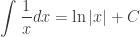 . The absolute value sign is to remind you that the argument of the logarithm function must be positive, since in some situations x itself may be negative.
 and
and  .
. , times the thickness of the paint. As everyone knows paint is thin, specifically
  thin. So we add an amount of paint to the sphere equal to
  .
. . As usual
 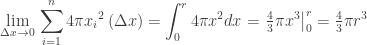 .
. , gains area at a rate equal to its perimeter times the “thickness of the edge”

 , times the “thickness of the face”
 . They are instructed to find the antiderivative, then tack on a +C , then substitute in the initial condition, then solve for C and finally write the particular solution. So we hope to see:


 , with an initial condition
  has the solution


 then, using the accumulation idea I’ve been discussing in my last few posts, its equation is


 at which point you are done; you have an equation of the line.
 and then substituting the coordinates of the point into the resulting equation, and then solving for b, and then writing the equation all over again, this time with only m and b substituted. It’s an algorithm. Okay, it’s short and easy enough to do, but why bother when you can have the equation in one step?
 .
.
