An Exploration in Differential Equations

Posted on January 18, 2019 by Lin McMullin

This is an exploration based on the AP Calculus question 2018 AB 6. I originally posed it for teachers last summer. This will make, I hope, a good review of many of the concepts and techniques students have learned during the year. The exploration, which will take an hour or more, includes these topics:

Finding the general solution of the differential equation by separating the variables
Checking the solution by substitution
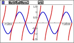
Using a graphing utility to explore the solutions for all values of the constant of integration, C
Finding the solutions’ horizontal and vertical asymptotes
Finding several particular solutions
Finding the domains of the particular solutions
Finding the extreme value of all solutions in terms of C
Finding the second derivative (implicit differentiation)
Considering concavity
Investigating a special case or two

I also hope that in working through this exploration students will learn not so much about this particular function, but how to use the tools of algebra, calculus, and technology to fully investigate any function and to find all its foibles.

The exploration is here in a PDF file. Here are the solutions.

As always, I appreciate your feedback and comments. Please share them with me using the reply box below.

The College Board is pleased to offer a new live online event for new and experienced AP Calculus teachers on March 5th at 7:00 PM Eastern.

I will be the presenter.

The topic will be AP Calculus: How to Review for the Exam: In this two-hour online workshop, we will investigate techniques and hints for helping students to prepare for the AP Calculus exams. Additionally, we’ll discuss the 10 type questions that appear on the AP Calculus exams, and what students need know and to be able to do for each. Finally, we’ll examine resources for exam review.

Registration for this event is $30/members and $35/non-members. You can register for the event by following this link: http://eventreg.collegeboard.org/d/xbqbjz

The Mean Value Theorem

Posted on October 23, 2018 by Lin McMullin

Another application of the derivative is the Mean Value Theorem (MVT). This theorem is very important. One of its most important uses is in proving the Fundamental Theorem of Calculus (FTC), which comes a little later in the year.

See last Fridays post Foreshadowing the MVT for an a series of problems that will get your students ready for the MVT.

Here are some previous post on the MVT:

Fermat’s Penultimate Theorem A lemma for Rolle’s Theorem: Any function extreme value(s) on an open interval must occur where the derivative is zero or undefined.

Rolle’s Theorem A lemma for the MVT: On an interval if a function is continuous on a closed interval [a, b] and differentiable on the open interval (a, b) and f(a) = f(b), there must exist a number c in the open interval (a, b) where f ‘(c) = 0.

Mean Value Theorem I Proof

Mean Value Theorem II Graphical Considerations

Darboux’s Theorem The Intermediate Value Theorem for derivatives.

Mean Tables

Revised from a post of October 31, 2017

Foreshadowing the MVT

Posted on October 19, 2018 by Lin McMullin

The Mean Value Theorem (MVT) is proved by writing the equation of a function giving the (directed) length of a segment from the given function to the line between the endpoints as you can see here. Since the function and the line intersect at the endpoints of the interval this function satisfies the hypotheses of Rolle’s theorem and so the MVT follows directly. This means that the derivative of the distance function is zero at the points guaranteed by the MVT. Therefore, these values must also be the location of the local extreme values (maximums and minimums) of the distance function on the open interval. *

Here is an exploration with three similar examples that use this idea to foreshadow the MVT. You, of course, can use your own favorite function. Any differentiable function may be used, in which case a CAS calculator may be helpful. Answers are at the end.

First example:

Consider the function $f(x)=x+2\sin (\pi x)$ defined on the closed interval [–1,3]

Write the equation of the line through the endpoints of the function.
Write an expression for h(x) the vertical distance between f(x) and the line found in part 1.
Find the x-coordinates of the local extreme values of h(x) on the open interval (–1,3).
Find the slope of f(x) at the values found in part 3.
Compare your answer to part 4 with the slope of the line. Is this a coincidence?

Second example: slightly more difficult than the first.

Consider the function $f\left( x \right)=1+x+2\cos \left( x \right)$ defined on the closed interval $\left[ {\tfrac{\pi }{2},\tfrac{{9\pi }}{2}} \right]$

Write the equation of the line through the endpoints of the function.
Write an expression for h(x) the vertical distance between f(x) and the line found in part 1.
Find the x-coordinates of the local extreme values of h(x) on the open interval $\left( {\tfrac{\pi }{2},\tfrac{{9\pi }}{2}} \right)$
Find the slope of f(x) at the values found in part 3.
Compare your answer to part 4 with the slope of the line. Is this a coincidence?

Third example: In case you think I cooked the numbers

Consider the function $\displaystyle f(x)={{x}^{3}}$ defined on the closed interval $\displaystyle [-4.5]$

Write the equation of the line thru the endpoints of the function.
Write an expression for h(x) the vertical distance between f(x) and the line found in part 1.
Find the x-coordinates of the local extreme values of h(x) on the open interval $\displaystyle (-4,5)$
Find the slope of f(x) at the values found in part 3.
Compare your answer to part 4 with the slope of the line. Is this a coincidence?

Answers

First example:

y = x
$\displaystyle h(x)=f(x)-y(x)=\left( {x+2\sin (\pi x)} \right)-\left( x \right)=2\sin (\pi x)$
${h}'\left( x \right)=2\pi \cos \left( {\pi x} \right)=0$ when x = –1/2, ½, 3/2 and 5/2
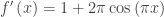
$\displaystyle {f}'\left( x \right)=1+2\pi \cos \left( {\pi x} \right)$ , the slope = 1 at all four points
They are the same. Not a coincidence.

Second example:

The endpoints are $\left( {\tfrac{\pi }{2},1+\tfrac{\pi }{2}} \right)$ and $\left( {\tfrac{{9\pi }}{2},1+\tfrac{{9\pi }}{2}} \right)$ ; the line is $y=x+1$
$h\left( x \right)=f\left( x \right)-y\left( x \right)=\left( {1+x+2\cos (x)} \right)-\left( {x+1} \right)=2\cos \left( x \right)$
${h}'\left( x \right)-2\sin (x)=0$ when $x=\pi ,2\pi ,3\pi ,\text{ and }4\pi$
${f}'\left( x \right)=1-2\sin \left( x \right)$ , at the points above the slope is 1.
They are the same. Not a coincidence.

Third example:

The endpoints are (-4, -64) and (5, 125), the line is $\displaystyle y=125+21(x-5)=21x+20$
$\displaystyle h(x)={{x}^{3}}-21x-20$
$\displaystyle {h}'(x)=3{{x}^{2}}-21=0$ when $\displaystyle x=\sqrt{7},-\sqrt{7}$
$\displaystyle {f}'\left( {\pm \sqrt{7}} \right)=3{{\left( {\pm \sqrt{7}} \right)}^{2}}=21$
They are the same. Not a coincidence.

* It is possible that the derivative is zero and the point is not an extreme value. This is similar to the situation with a point of inflection when the first derivative is zero but does not change sign.

Teaching Concavity

Posted on October 17, 2018 by Lin McMullin

As you’ve probably noticed, different authors use different definitions based on how they plan to present topics later in their texts. So, the same concept seems to have different definitions. A definition in one book is a theorem in another. Students should be aware of this; looking at different definitions and related theorems about the same idea helps their mathematical education.

Here is a thought on exploring how concepts may be defined and learning about concavity are the same time.

Start by drawing the 4 shapes of (non-linear) graphs (See Concepts Related to Graphs and The Shapes of a Graph.)

Increasing, concave up
Increasing concave down
Decreasing concave up
Decreasing concave down

Look at the sine or cosine graphs which show all four and the tangent graph that shows only two. Look at other functions as well and identify which parts (intervals) exhibit each shape.

Next, challenge the students, in groups, individually, in class, or for homework to find analytic ways to say what concavity is or to identify it from equations. If they need hints suggest they look at derivatives (first and second) and tangent lines. Don’t limit them – explain that there are other ways. They should try to find several ways.

Hopefully, they will come up with some of these. (I have purposely listed these in a rough preliminary form. That’s how math is done – get an idea and then develop and formalize it)

A function is concave up (down) when:

The slope (derivative) is increasing (decreasing)
The second derivative is positive (negative).
The tangent line lies below (above) the graph
All (any, every) segments joining points in the interval lie above (below) the graph.
Others ???

Finally, clean these up. Help the students:

State them as “if, then” or “if, and only if” statements giving the hypotheses for each.
Consider how one can be used to imply the others – in either direction.
Determine which implies the inclusion of endpoints (1 and maybe 3).
Discuss which the class thinks would make the best definition, and which should become theorems.
Taking whichever definition your book uses, show how the others can be proved.

The point here is the thinking, forming ideas, doing the mathematics; the understanding of concavity will follow.

L’Hospital’s Rule

Posted on October 16, 2018 by Lin McMullin

Another application of the derivative

L’Hospital’s Rule

Locally Linear L’Hospital’s Demonstration of the proof

L’Hospital Rules the Graph

Good Question An AP Exam question that can be used to delve deeper into L’Hospital’s Rule (2008 AB 6)

Guillaume de l’Hospital
1661 – 1704

Revised from a post of November 7, 2017

There will be two extra posts this week! Check tomorrow for some suggestions on “Teaching Concavity” and on Friday for “Foreshadowing the MVT.”

I made a major update to last Friday’s post On Scaling. It includes a suggestion from a reader of this blog with a Desmos graph that will calculate the Kennedy scale scores for you.

Graphing – an Application of the Derivative.

Posted on October 9, 2018 by Lin McMullin

Graphing and the analysis of graphs given (1) the equation, (2) a graph, or (3) a table of values of a function and its derivative(s) makes up the largest group of questions on the AP exams. Most of the other applications of the derivative depend on understanding the relationship between a function and its derivatives.