Inverses

This series of posts reviews and expands what students know from pre-calculus about inverses. This leads to finding the derivative of exponential functions, ax, and the definition of e, from which comes the definition of the natural logarithm.

Inverses Graphically and Numerically

The Range of the Inverse

The Calculus of Inverses

The Derivatives of Exponential Functions and the Definition of e and This pair of posts shows how to find the derivative of an exponential function, how and why e is chosen to help this differentiation.

Logarithms Inverses are used to define the natural logarithm function as the inverse of ex. This follow naturally from the work on inverses. However, integration is involved and this is best saved until later. I will mention it then.

Two new post coming soon:

Implicit Differentiation

Often a relation (an expression in x and y), that has a graph but is not a function, needs to be analyzed. But the relation is not or cannot be solved for y. What to do? The answer is to use the technique of implicit differentiation. Assume there is a way to solve for y and differentiate using the Chain Rule. Whenever you get to the y,“differentiate” it by writing dy/dx. Then solve for dy/dx

Here are several previous posts on this topic and how to go about using it.

Implicit Differentiation

Implicit Differentiation and Inverses

Implicit differentiation of parametric equations   These are BC topics

A Vector’s Derivative  These are BC topics

_____________________________________________________

The Chain Rule

Most of the function students are faced with in beginning calculus are compositions of the Elementary Functions. The Chain Rule allows you to differentiate composite functions easily. The posts listed below are ways to introduce and use the Chain Rule.

Experimenting with a CAS – Chain Rule  Using a CAS to discover the Chain Rule

Power Rule Implies Chain Rule and Foreshadowing the Chain Rule the same ideas.

The Chain Rule


Revised from 9-19-2017

Derivative Formulae

Maria Gaetana Agnesi

So, no one wants to do complicated limits to find derivatives. There are easier ways of course. There are a number of quick ways (rules, formulas) for finding derivatives of the Elementary Functions and their compositions. Here are some ways to introduce these rules; these are the subject of this week’s review of past posts.

Why Radians?

The Derivative I        Guessing the derivatives from the definition

The Derivative II      Using difference quotients to graph and guess

The Derivative Rules I    The Power Rule

The Derivative Rules II       Another approach to the Product Rule from my friend Paul Foerster

The Derivative Rules III     The Quotient Rule developed using the Power Rule, an approach first suggested  by Maria Gaetana Agnesi (1718 – 1799) who was helping her brother learn the calculus.

Next week: The Chain Rule.


Revised from 9-12-2017

Difference Quotients

Difference quotients are the path to the definition of the derivative. Here are three posts exploring difference quotients.

Difference Quotients I  The forward and backward difference quotients

Difference Quotients II      The symmetric difference quotient and seeing the three difference quotients in action.  Showing that the three difference quotients converge to the same value.

Seeing Difference Quotients      Expands on the post immediately above and shows some numerical and graphical approaches using calculators or the Desmos graph

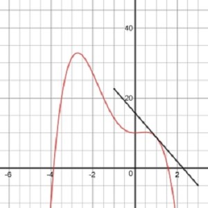
 Tangents and Slopes You can use this Desmos app now to preview some of the things that he tangent line can tell us about the graph of a function or save (or reuse) it for later when concentrating on graphs. Discuss slope in relation to increasing, decreasing, concavity, etc.

At Just the Right Time

Stamp out Slope-intercept Form


Updated from a post of 9-5-2017


Local Linearity

If you use your calculator or graphing program and zoom-in of the graph of a function (with equal zoom factors in both directions), the graph eventually looks like a line: the graph appears to be straight. This property is called Local Linearity. The slope of this line is the number called the derivative. (There are exceptions: if the graph never appears linear, then no derivative exists at that point.) Local Linearity is the graphical manifestation of differentiability. 

To find this slope, we need to zoom-in numerically. Zooming-in numerically is accomplished by finding the slope of a secant line, a line that intersects the graph twice near the point we are interested in. Then finding the limit of that slope as the two points come closer to our point. This limit is the derivative. It is also the slope of the line tangent to the function at the point. 

While limit is what makes all of the calculus work, people usually think of calculus as starting with the derivative. The first problem in calculus is finding the slope of a line tangent to a graph at a point and then writing the equation of that tangent line. The slope is called the derivative and a function whose derivative exists is said to be differentiable. 

This week’s posts start with local linearity and tangent lines. They lead to the difference quotient and the equation of the tangent line.

Local Linearity I

Local Linearity II      Working up to difference quotient. The next post explains this in more detail.

Tangent Lines approaching difference quotients on calculator by graphing tan line.

Next week: Difference Quotients.


Revised from a post of August 29, 2017


Summer Fun

Every Spring I have a lot of fun proofreading Audrey Weeks’ new Calculus in Motion illustrations for the most recent AP Calculus Exam questions. These illustrations run on Geometers’ Sketchpad. In addition to the exam questions Calculus in Motion (and its companion Algebra in Motion) include separate animations illustrating most of the concepts in calculus and algebra. This is a great resource for your classes.

The proofreading and the cross-country conversations with Audrey give me a chance to learn more about the questions.

This year, I really got into 2018 AB 6, the differential equation question. I wrote an exploration (or as the kids would say “worksheet”) on a function very similar to the differential equation in that question. The exploration, which is rather long, includes these topics:

  • Finding the general solution of the differential equation by separating the variables
  • Checking the solution by substitution
  • Using a graphing utility to explore the solutions for all values of the constant of integration, C
  • Finding the solutions’ horizontal and vertical asymptotes
  • Finding several particular solutions
  • Finding the domains of the particular solutions
  • Finding the extreme value of all solutions in terms of C
  • Finding the second derivative (implicit differentiation)
  • Considering concavity
  • Investigating a special case or two

I also hope that in working through this exploration students will learn not so much about this particular function, but how to use the tools of algebra, calculus, and technology to fully investigate any function and to find all its foibles.

Students will need to have studied calculus through differential equations before they start the exploration. I will repost it next January for them.

The exploration is here for you to try. Try it before you look at the solutions. It will give you something to do over the summer – well not all summer, only an hour or so.

As always, I appreciate your feedback and comments. Please share them with me using the reply box below.


There will be only occasional, very occasional, posts over the Summer. More regular posting will begin again in August. Enjoy the Explorations, and, more important, enjoy the Summer!

.