Rate & Accumulation (Type 1)

Posted on March 11, 2022 by Lin McMullin

The Free-response Questions

There are ten general types of AP Calculus free-response questions. This and the next nine posts will discuss each of them.

NOTE: The numbers I’ve assigned to each type DO NOT correspond to the CED Unit numbers. Many AP Exam questions intentionally have parts from different Units. The CED Unit numbers will be referenced in each post.

AP Questions Type 1: Rate and Accumulation

These questions are often in context with a lot of words describing a situation in which some quantities are changing. There are usually two rates acting in opposite ways (sometimes called an in-out question). Students are asked about the change that the rates produce over a time interval either separately or together.

The rates are often fairly complicated functions. If the question is on the calculator allowed section, students should store the functions in the equation editor of their calculator and use their calculator to do any graphing, integration, or differentiation that may be necessary.

The main idea is that over the time interval [a, b] the integral of a rate of change is the net amount of change

$\displaystyle \int_{a}^{b}{{{f}'\left( t \right)dt}}=f\left( b \right)-f\left( a \right)$

If the question asks for an amount, look around for a rate to integrate.

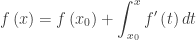
The final (accumulated) amount is the initial amount plus the accumulated change:

$\displaystyle f\left( x \right)=f\left( {{{x}_{0}}} \right)+\int_{{{{x}_{0}}}}^{x}{{{f}'\left( t \right)dt}}$

where $\displaystyle {{x}_{0}}$ is the initial time, and $\displaystyle f\left( {{{x}_{0}}} \right)$ is the initial amount. Since this is one of the main interpretations of the definite integral the concept may come up in a variety of situations.

What students should be able to do:

Be ready to read and apply; often these problems contain a lot of words which need to be carefully read and understood.
Understand the question. It is often not necessary to do as much computation as it seems at first.
Recognize that rate = derivative.
Recognize a rate from the units given without the words “rate” or “derivative.”
Find the change in an amount by integrating the rate. The integral of a rate of change gives the amount of change (FTC):

$\displaystyle \int_{a}^{b}{{{f}'\left( t \right)dt}}=f\left( b \right)-f\left( a \right)$

Find the final amount by adding the initial amount to the amount found by integrating the rate. If $\displaystyle {{x}_{0}}$ is the initial time, and $\displaystyle f\left( {{{x}_{0}}} \right)$ is the initial amount, then final accumulated amount is

$\displaystyle f\left( x \right)=f\left( {{{x}_{0}}} \right)+\int_{{{{x}_{0}}}}^{x}{{{f}'\left( t \right)dt}}$ ,

Write an integral expression that gives the amount at a general time. BE CAREFUL, the dt must be included in the correct place. Think of the integral sign and the dt as parentheses around the integrand.
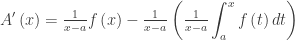
Find the average value of a function
Use FTC to differentiate a function defined by an integral.
Explain the meaning of a derivative or its value in terms of the context of the problem. The explanation should contain (1) what it represents, (2) its units, and (3) what the numerical argument means in the context of the question.
Explain the meaning of a definite integral or its value in terms of the context of the problem. The explanation should contain (1) what it represents, (2) its units, and (3) how the limits of integration apply in the context of the question.
Store functions in their calculator recall them to do computations on their calculator.
If the rates are given in a table, be ready to approximate an integral using a Riemann sum or by trapezoids. Also, be ready to approximate a derivative using a quotient from the numbers in the table.
Do a max/min or increasing/decreasing analysis.

Shorter questions on this concept appear in the multiple-choice sections. As always, look over as many questions of this kind from past exams as you can find.

The Rate – Accumulation question may cover topics primarily from Unit 4, Unit 5, Unit 6 and Unit 8 of the CED.

Typical free-response examples:

2013 AB1/BC1
2015 AB1/BC1
2018 AB1/BC1
2019 AB1/BC1
2022 AB1/BC1 – includes average value, inc/dec analysis, max/min analysis
2023 AB1/BC1 – Table stem, average value, MVT,
One of my favorites Good Question 6 (2002 AB 4)

Typical multiple-choice examples from non-secure exams:

2012 AB 8, 81, 89
2012 BC 8 (same as AB 8)

Updated January 31, 2019, March 12, 2021, March 11, 2022. February 17, 2024

Extreme Average

Posted on January 4, 2022 by Lin McMullin

A recent post on the AP Calculus bulletin board observed that the maximum value of the average value of a function on an interval occurred at the point where the graph of the average value and the function intersect. I am not sure if this concept is important in and of itself, but it does make an interesting exercise.

For a function f(x), we may treat its average value as a function, A(x), defined for all x ∈ [a, b], interval [a, x] as

$\displaystyle A\left( x \right)=\left\{ {\begin{array}{*{20}{c}} {\tfrac{1}{{x-a}}\int_{a}^{x}{{f\left( t \right)dt}}} & {x\ne a} \\ {f\left( a \right)} & {x=a} \end{array}} \right.$

Graphically, the segment drawn at y = A(x) is such that the regions between the line and the function above and below the segment have equal areas. See figure 1 in which the red curve is the function, and the blue curve is the average value function. The two shaded regions have the same area.

Figure 1: The shaded regions have the same area.

Regardless of the starting value, the function and its average value start at the same value. If the function is increasing the average value is less than the function and increasing. When the function starts to decrease, the average value will continue to increase for a while. When the two graphs nest intersect, the process starts over, and the average value will now start to decrease. Therefore, the intersection value is when the average value function change from increasing to decreasing and this is its (local) maximum value. See Figure 2.

Figure 2:The maximum value of A(x) is at the intersection of the two graphs

This continues until the graphs intersect again after the function starts to increase: a (local) minimum value of the average value function. The process continues with the extreme values of the average value function (blue graph) occurring at its intersections with the function. Figure 3

Figure 3: A(x) has its extreme values where it intersects the function.

This can be proved by finding the extreme values of the average value function by considering its derivative. Begin by finding its derivative using the product rule (or quotient rule) and the FTC.

$\displaystyle {A}'\left( x \right)=\tfrac{1}{{x-a}}f\left( x \right)+\left( {-\tfrac{1}{{{{{\left( {x-a} \right)}}^{2}}}}} \right)\int_{a}^{x}{{f\left( t \right)dt}}$

$\displaystyle {A}'\left( x \right)=\tfrac{1}{{x-a}}f\left( x \right)-\tfrac{1}{{x-a}}\left( {\tfrac{1}{{x-a}}\int_{a}^{x}{{f\left( t \right)dt}}} \right)$

$\displaystyle {A}'\left( x \right)=\tfrac{1}{{x-a}}\left( {f\left( x \right)-A\left( x \right)} \right)$

The critical points of a(x) occur when its derivative is equal to zero (or undefined). This is when $f\left( x \right)=A\left( x \right)$ (or when x = a, the endpoint). This is where the graphs intersect.

How to use this in your class

This is not a concept that is likely to be tested on the AP Calculus Exams. Nevertheless, it is an easy enough idea to explore when teaching the average value of a function and at the same time reviewing some earlier concepts such as product (or quotient) rule, the FTC (differentiating an integral), and some non-ordinary simplification.

You could have your students use their own favorite function and show that the extreme values of its average value occur where the average value intersects the function. This is good practice in equation solving on a calculator since the points do not occur at “nice” numbers. Here’s an example.

If $\displaystyle f\left( x \right)=\sin \left( x \right)$ , then its average value on the interval $\displaystyle [0,\infty )$ is

$\displaystyle A\left( x \right)=\tfrac{1}{x}\int_{0}^{x}{{\sin \left( t \right)dt}}=\frac{{-\cos \left( x \right)+1}}{x}$ .

The intersections of f(x) and A(x) can be found by solving

$\displaystyle\sin \left( x \right)=\frac{{-\cos \left( x \right)+1}}{x}$

The extreme values of $\displaystyle \frac{{-\cos \left( x \right)+1}}{x}$ may also be found using a calculator.

The points are the same. the first is approximately (2.331, 0.725) and the second is (6.283, 0) or (2π, 0). This second is reasonable since at 2π the sine function has completed one period and its average value zero. (See figure 3 again.).

Other questions you could ask (for my function anyway) are what is the absolute maximum and how can you be sure? Why are all the minimums zero?

The message on the AP Calculus discussion boards that inspired this post was started by Neema Salimi an AP Calculus teacher from Georgia. He made the original observation. You can read his original post and proof, and comments by others here.

The Rule of Four

Not much has been heard of the Rule of Four lately. The Rule of Four suggests that mathematical concepts should be looked at graphically, numerically, analytically, and verbally. It has not gone away. The Rule of Four has a new name: multiple representations. (In the latest Course and Exam Description, you will find it in Mathematical Practices (p. 14), specifically practices 2.B, 2.C, 2.D, 2.E, 3.E, 3.F, 4.A, and 4.C)

I have used the Rule of Four in this post. The post started with a verbal discussion of the concept and how the result can be seen graphically. That was followed by analytic proof. At the end is a numerical example.

Other posts on the average value of a function:

Finding the average value of a function on an interval is Topic 8.1 in the Course and Exam Description (p. 149)

Average Value of a Function – or How do you average an infinite number of numbers?

Most Triangles Are Obtuse! An obvious observation, but here’s how to figure the exact proportion of obtuse to acute triangles.

Half-full or Half-empty Visualizing the average value of a function

What’s a Mean Old Average Anyway? Be sure to distinguish between the average rate of change, the average value of a function, and the mean value theorem.

Open or Closed?

Posted on October 26, 2021 by Lin McMullin

About this time of year, you find someone, hopefully one of your students, asking, “If I’m finding where a function is increasing, is the interval open or closed?”

Do you have an answer?

This is a good time to teach some things about definitions and theorems.

The place to start is to ask what it means for a function to be increasing. Here is the definition:

A function is increasing on an interval if, and only if, for all (any, every) pairs of numbers x₁ < x₂ in the interval, f(x₁) < f(x₂).”

(For decreasing on an interval, the second inequality changes to f(x₁) > f(x₂). All of what follows applies to decreasing with obvious changes in the wording.)

Notice that functions increase or decrease on intervals, not at individual points. We will come back to this in a minute.
Numerically, this means that for every possible pair of points, the one with the larger x-value always produces a larger function value.
Graphically, this means that as you move to the right along the graph, the graph is going up.
Analytically, this means that we can prove the inequality in the definition.

For an example of this last point consider the function f(x) = x². Let x₂= x₁ + h where h > 0. Then in order for f(x₁) < f(x₂) it must be true that

$\displaystyle {{x}_{1}}^{2}<{{\left( {{{x}_{1}}+h} \right)}^{2}}$

$\displaystyle 0<{{\left( {{{x}_{1}}+h} \right)}^{2}}-{{x}_{1}}^{2}$

$\displaystyle 0<{{x}_{1}}^{2}+2{{x}_{1}}h+{{h}^{2}}-{{x}_{1}}^{2}$

$\displaystyle 0<2{{x}_{1}}h+{{h}^{2}}$

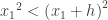
This can only be true if $\displaystyle {{x}_{1}}\ge 0$ Thus, x² is increasing only if $\displaystyle {{x}_{1}}\ge 0$

Now, of course, we rarely, if ever, go to all that trouble. And it is even more trouble for a function that increases on several intervals. The usual way of finding where a function is increasing is to look at its derivative.

Notice that the expression $\displaystyle 0<{{x}_{1}}^{2}+2{{x}_{1}}h+{{h}^{2}}-{{x}_{1}}^{2}$ looks a lot like the numerator of the original limit definition of the derivative of x² at x = x₁, namely $\displaystyle 0<{{\left( {{{x}_{1}}+h} \right)}^{2}}-{{x}_{1}}^{2}$ . If h > 0, where the function is increasing the numerator is positive and the derivative is positive also. Turning this around we have a theorem that says, If $\displaystyle {f}'\left( {{{x}_{1}}} \right)>0$ for all x in an interval, then the function is increasing on the interval. That makes it much easier to find where a function is increasing, we simplify find where its derivative is positive.

There is only a slight problem in that the theorem does not say what happens if the derivative is zero somewhere on the interval. If that is the case, we must go back to the definition of increasing on an interval or use a different method. For example, the function x³ is increasing everywhere, even though its derivative at the origin is zero.

Let’s consider another example. The function sin(x) is increasing on the interval $\displaystyle [-\tfrac{\pi }{2},\tfrac{\pi }{2}]$ (among others) and decreasing on $\displaystyle [\tfrac{\pi }{2},\tfrac{3\pi }{2}]$ . It bothers some that $\displaystyle \tfrac{\pi }{2}$ is in both intervals and that the derivative of the function is zero at x = $\displaystyle \tfrac{\pi }{2}$ . This is not a problem. Sin( $\displaystyle \tfrac{\pi }{2}$ ) is larger than all the other values is both intervals, so by the definition, and not the theorem, the intervals are correct.

It is generally true that if a function is continuous on the closed interval [a,b] and increasing on the open interval (a,b) then it must be increasing on the closed interval [a,b] as well.

Returning to the first point above: functions increase or decrease on intervals not at points. You do find questions in books and on tests that ask, “Is the function increasing at x = a.” The best answer is to humor them and answer depending on the value of the derivative at that point. Since the derivative is a limit as h approaches zero, the function must be defined on some interval around x = a in which h is approaching zero. So, answer according to the value of the derivative on that interval.

You can find more on this here.

Case Closed.

Slightly revised from a posted published on November 2, 2012.

Extreme Values

Posted on October 22, 2021 by Lin McMullin

Every function that is continuous on a closed interval must have a maximum and a minimum value on the interval. These values may all be the same (y = 2 on [-3,3]); or the function may reach these values more than once (y = sin(x)).

If the function is defined on a closed interval, then the extreme values are either (1) at an endpoint of the interval or (2) at a critical number. This is known as the Extreme Value Theorem. Thus, one way of finding the extreme values is to simply find the value of the function at the endpoints and the critical points and compare these to find the largest and smallest. This is called the Candidates’ Test or the Closed Interval Test. It is a good one to “play” with: do some sketches of the different situation above; discuss why the interval must be closed.

On an open or closed interval, the shapes can change if the first derivative is zero or undefined at the point where two shapes join. In this case the point is a local extreme value of the function – a local maximum or minimum value. Specifically:

If the first derivative changes from positive to negative, the shape of the function changes from increasing to decreasing and the point is a local maximum. If the first derivative changes from negative to positive, the shape of the function changes from decreasing to increasing and the point is a local minimum.

This is a theorem called the First Derivative Test. By finding where the first derivative changes sign and in which direction it changes (positive to negative, or negative to positive) we can locate and identify the local extreme value precisely.

Another way to determine if a critical number is the location of a local maximum or minimum is a theorem called the Second Derivative Test.

If the first derivative is zero (and specifically not if it is undefined) and the second derivative is positive, then the graph has a horizontal tangent line and is concave up. Therefore, this is the location of a local minimum of the function.

Likewise, if the first derivative is zero at a point and the second derivative is negative there, the function has a local maximum there.

If both the first and second derivatives are zero at a point, then the second derivative test cannot be used, for example y = x⁴ at the origin.

The mistake students make with the second derivative test is in not checking that the first derivative is zero. If “justify your answer” is required, students should be sure to show that the first derivative is zero as well as the sign of the second derivative.

In the case where both the first and second derivatives are zero at the same point the function changes direction but not concavity (e.g. f (x) = x⁴at the origin), or changes concavity but not direction (e.g. f (x) = x³at the origin).

This is a revised version of a post published on October 22, 2012

Reading the Derivative’s Graph

Posted on October 19, 2021 by Lin McMullin

A very typical calculus problem is given the equation of a function, to find information about it (extreme values, concavity, increasing, decreasing, etc., etc.). This is usually done by computing and analyzing the first derivative and the second derivative. All the textbooks show how to do this with copious examples and exercises. I have nothing to add to that. One of the “tools” of this approach is to draw a number line and mark the information about the function and the derivative on it.

A very typical AP Calculus exam problem is given the graph of the derivative of a function, but not the equation of either the derivative or the function, to find all the same information about the function. For some reason, students find this difficult even though the two-dimensional graph of the derivative gives all the same information as the number line graph and, in fact, a lot more.

Looking at the graph of the derivative in the x,y-plane it is easy to determine the important information. Here is a summary relating the features of the graph of the derivative with the graph of the function.

Feature	the function
${y}'$ > 0	is increasing
${y}'$ < 0	is decreasing
${y}'$ changes – to +	has a local minimum
${y}'$ changes + to –	has a local maximum
${y}'$ increasing	is concave up
${y}'$ decreasing	is concave down
${y}'$ extreme value	has a point of inflection

Here’s a typical graph of a derivative with the first derivative features marked.

Here is the same graph with the second derivative features marked.

The AP Calculus Exams also ask students to “Justify Your Answer.” The table above, with the columns switched does that. The justifications must be related to the given derivative, so a typical justification might read, “The function has a relative maximum at x = -2 because its derivative changes from positive to negative at x = -2.”

Conclusion	Justification
y is increasing	${y}'$ > 0
y is decreasing	${y}'$ < 0
y has a local minimum	${y}'$ changes – to +
y has a local maximum	${y}'$ changes + to –
y is concave up	${y}'$ increasing
y is concave down	${y}'$ decreasing
y has a point of inflection	${y}'$ extreme values

For notes on asymptotes see Asymptotes and the Derivative and Other Asymptotes.

Originally posted on October 26, 2012, and my single most viewed post over the years.

Foreshadowing the MVT

Posted on October 15, 2021 by Lin McMullin

The Mean Value Theorem (MVT) is proved by writing the equation of a function giving the (directed) length of a segment from the given function to the line between the endpoints as you can see here. Since the function and the line intersect at the endpoints of the interval this function satisfies the hypotheses of Rolle’s theorem and so the MVT follows directly. This means that the derivative of the distance function is zero at the points guaranteed by the MVT. Therefore, these values must also be the location of the local extreme values (maximums and minimums) of the distance function on the open interval. *

Here is an exploration in three similar examples that use this idea to foreshadow the MVT. You, of course, can use your own favorite function. Any differentiable function may be used, in which case a CAS calculator may be helpful. Answers are at the end.

First example:

Consider the function $\displaystyle f\left( x \right)=x+2\sin \left( {\pi x} \right)$ defined on the closed interval [–1,3]

Write the equation of the line thru the endpoints of the function.
Write an expression for h(x) the vertical distance between f(x) and the line found in part 1.
Find the x-coordinates of the local extreme values of h(x) on the open interval (–1,3).
Find the slope of f(x) at the values found in part 3.
Compare your answer to part 4 with the slope of the line. Is this a coincidence?

Second example: slightly more difficult than the first.

Consider the function $\displaystyle f\left( x \right)=1+x+2\cos (x)$ defined on the closed interval $\displaystyle [\tfrac{\pi }{2},\tfrac{{9\pi }}{2}]$ .

Write the equation of the line thru the endpoints of the function.
Write an expression for h(x) the vertical distance between f(x) and the line found in part 1.
Find the x-coordinates of the local extreme values of h(x) on the open interval $\displaystyle \left( {\tfrac{\pi }{2},\tfrac{{9\pi }}{2}} \right)$ .
Find the slope of f(x) at the values found in part 3.
Compare your answer to part 4 with the slope of the line. Is this a coincidence?

Third example: In case you think I cooked the numbers. You may want to use a CAS for this one.

Consider the function $\displaystyle f(x)={{x}^{3}}$ defined on the closed interval $\displaystyle [-4,5]$ .

Write the equation of the line thru the endpoints of the function.
Write an expression for h(x) the vertical distance between f(x) and the line found in part 1.
Find the x-coordinates of the local extreme values of h(x) on the open interval $\displaystyle \left( {-4,5} \right)$ .
Find the slope of f(x) at the values found in part 3.
Compare your answer to part 4 with the slope of the line. Is this a coincidence?

Answers

First example:

y = x
$\displaystyle h(x)=f(x)-y(x)=x-\left( {x+2\sin (\pi x} \right)=\left( {2\sin (\pi x} \right)$
$\displaystyle {h}'\left( x \right)=2\pi \cos \left( {\pi x} \right)=0$ when x = –1/2, ½, 3/2 and 5/2
$\displaystyle {f}'\left( x \right)=1+2\pi \cos \left( {\pi x} \right)=1$ , the slope = 1 at all four points
They are the same. Not a coincidence.

Second example:

The endpoints are $\displaystyle \left( {\tfrac{\pi }{2},1+\tfrac{\pi }{2}} \right)$ and $\displaystyle \left( {\tfrac{9\pi }{2},1+\tfrac{{9\pi }}{2}} \right)$ ; the line is $\displaystyle y=x+1$
$\displaystyle h(x)=f(x)-y(x)=\left( {1+x+2\cos (x)} \right)-(x+1)=2\cos (x)$
$\displaystyle {h}'\left( x \right)=-2\sin (x)=0$ when $\displaystyle x=\pi ,2\pi ,3\pi ,\text{ and }4\pi$
$\displaystyle {f}'\left( x \right)=1-2\sin \left( x \right)=1$ ; at the points above the slope is 1.
They are the same. Not a coincidence.

Third example:

The endpoints are (-4, -64) and (5, 125), the line is $\displaystyle y=125+21\left( {x-5} \right)=21x+20$ .
$\displaystyle h\left( x \right)={{x}^{3}}-21x-20$
$\displaystyle {h}'\left( x \right)=3{{x}^{2}}-21=0$ when $\displaystyle x=\sqrt{7},-\sqrt{7}$
$\displaystyle {f}'\left( {\pm \sqrt{7}} \right)=3{{\left( {\pm \sqrt{7}} \right)}^{2}}=21$
They are the same. Not a coincidence.

See this post for links to other posts discussing the full development of the MVT

* It is possible that the derivative is zero and the point is not an extreme value. This is like the situation with a point of inflection when the first derivative is zero but does not change sign.

This post was originally published on October 19, 2018.

Unit 5 – Analytical Applications of Differentiation

Posted on October 12, 2021 by Lin McMullin

Unit 5 covers the application of derivatives to the analysis of functions and graphs. Reasoning and justification of results are also important themes in this unit. (CED – 2019 p. 92 – 107). These topics account for about 15 – 18% of questions on the AB exam and 8 – 11% of the BC questions.

You may want to consider teaching Unit 4 after Unit 5. Notes on Unit 4 are here.

Reasoning and writing justification of results are mentioned and stressed in the introduction to the topic (p. 93) and for most of the individual topics. See Learning Objective FUN-A.4 “Justify conclusions about the behavior of a function based on the behavior of its derivatives,” and likewise in FUN-1.C for the Extreme value theorem, and FUN-4.E for implicitly defined functions. Be sure to include writing justifications as you go through this topic. Use past free-response questions as exercises and also as guide as to what constitutes a good justification. Links in the margins of the CED are also helpful and give hints on writing justifications and what is required to earn credit. See the presentation Writing on the AP Calculus Exams and its handout

Topics 5.1

Topic 5.1 Using the Mean Value Theorem While not specifically named in the CED, Rolle’s Theorem is a lemma for the Mean Value Theorem (MVT). The MVT states that for a function that is continuous on the closed interval and differentiable over the corresponding open interval, there is at least one place in the open interval where the average rate of change equals the instantaneous rate of change (derivative). This is a very important existence theorem that is used to prove other important ideas in calculus. Students often confuse the average rate of change, the mean value, and the average value of a function – See What’s a Mean Old Average Anyway?

Topics 5.2 – 5.9

Topic 5.2 Extreme Value Theorem, Global Verses Local Extrema, and Critical Points An existence theorem for continuous functions on closed intervals

Topic 5.3 Determining Intervals on Which a Function is Increasing or Decreasing Using the first derivative to determine where a function is increasing and decreasing.

Topic 5.4 Using the First Derivative Test to Determine Relative (Local) Extrema Using the first derivative to determine local extreme values of a function

Topic 5.5 Using the Candidates’ Test to Determine Absolute (Global) Extrema The Candidates’ test can be used to find all extreme values of a function on a closed interval

Topic 5.6 Determining Concavity of Functions on Their Domains FUN-4.A.4 defines (at least for AP Calculus) When a function is concave up and down based on the behavior of the first derivative. (Some textbooks may use different equivalent definitions.) Points of inflection are also included under this topic.

Topic 5.7 Using the Second Derivative Test to Determine Extrema Using the Second Derivative Test to determine if a critical point is a maximum or minimum point. If a continuous function has only one critical point on an interval then it is the absolute (global) maximum or minimum for the function on that interval.

Topic 5.8 Sketching Graphs of Functions and Their Derivatives First and second derivatives give graphical and numerical information about a function and can be used to locate important points on the graph of the function.

Topic 5.9 Connecting a Function, Its First Derivative, and Its Second Derivative First and second derivatives give graphical and numerical information about a function and can be used to locate important points on the graph of the function.

Topics 5.10 – 5.11

Optimization is an important application of derivatives. Optimization problems as presented in most textbooks, begin with writing the model or equation that describes the situation to be optimized. This proves difficult for students, and is not “calculus” per se. Therefore, writing the equation has not been asked on AP exams in recent years (since 1983). Questions give the expression to be optimized and students do the “calculus” to find the maximum or minimum values. To save time, my suggestion is to not spend too much time writing the equations; rather concentrate on finding the extreme values.

Topic 5.10 Introduction to Optimization Problems

Topic 5.11 Solving Optimization Problems

Topics 5.12

Topic 5.12 Exploring Behaviors of Implicit Relations Critical points of implicitly defined relations can be found using the technique of implicit differentiation. This is an AB and BC topic. For BC students the techniques are applied later to parametric and vector functions.

Timing

Topic 5.1 is important and may take more than one day. Topics 5.2 – 5.9 flow together and for graphing they are used together; after presenting topics 5.2 – 5.7 spend the time in topics 5.8 and 5.9 spiraling and connecting the previous topics. Topics 5.10 and 5.11 – see note above and spend minimum time here. Topic 5.12 may take 2 days.

The suggested time for Unit 5 is 15 – 16 classes for AB and 10 – 11 for BC of 40 – 50-minute class periods, this includes time for testing etc.

Finally, were I still teaching, I would teach this unit before Unit 4. The linear motion topic (in Unit 4) are a special case of the graphing ideas in Unit 5, so it seems reasonable to teach this unit first. See Motion Problems: Same thing, Different Context

This is a re-post and update of the third in a series of posts from last year. It contains links to posts on this blog about the differentiation of composite, implicit, and inverse functions for your reference in planning. Other updated post on the 2019 CED will come throughout the year, hopefully, a few weeks before you get to the topic.

Previous posts on these topics include:

Then There Is This – Existence Theorems

What’s a Mean Old Average Anyway

Did He, or Didn’t He? History: how to find extreme values without calculus

Mean Value Theorem

Foreshadowing the MVT

Fermat’s Penultimate Theorem

Rolle’s theorem

The Mean Value Theorem I

The Mean Value Theorem II

Graphing

Concepts Related to Graphs